Unit – IV
Time Series Analysis
Q1) Explain the components of time series.
A1)
A time series is set of data collected at successive point in a time or over successive period of time.A time series is a collection of observations made sequentially through time.The interval between observations can be any time interval (hours within days, weeks, months, years, etc.).
Some examples of time series are:
a) An analysis of a single sequence of data is called univariate time-series
analysis.
b) An analysis of several sets of data for the same sequence of time periods is called multivariate time-series analysis or, more simply, multiple time-series analysis.
Utilities of time series:
1. It helps in understanding past behaviour and is useful for prediction of future.
2. It facilitates comparison.
3. The various components of time series are useful to study the effective change under each component.
4. The reasons for variation can be studied by comparing actual with expected results.
COMPONENT OF TIME SERIES-
Fluctuation in a time series is mainly due to four basic components.
1 Secular trend or trend (T).
2 Seasonal variation (S).
3 Cyclical variation or cyclic fluctuation (C).
4 Irregular or random moments (I).
Secular trend or trend (T)
Seasonal Variation
Cyclic Components:
Irregular Variation:
Irregular variations are fluctuations in time series that are short in duration, erratic in nature and follow no regularity in the occurrence pattern. These variations are also referred to as residual variations since by after trend, cyclical and seasonal variations. Irregular fluctuations result due to the occurrence of unforeseen events like: FLOODs, EARTHQUAKES, WARS, and FAMINES etc.
Q2) From the following data of wholesale prices of wheat for ten years construct index number taking a) 1998 as base and b) by chain base method

A2)
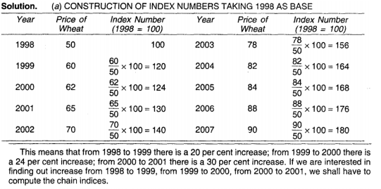
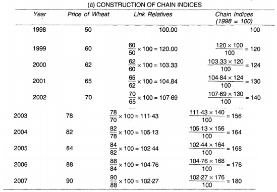
Q3) From the following data calculate the index numbers using the Chain Index Numbers method.
Year 2011 2012 2013 2014 2015 2016 2017 2018
Prices 120 124 130 144 150 160 164 170
A3)
Construction of Chain Index Numbers
Year | Price | Link Relatives | Chain indices |
2011 | 120 | 100 | 100 |
2012 | 124 | 120/124 x 100 = 103.33 | 103.33 ×100/100 = 103.33 |
2013 | 130 | 124/130 x 100 = 104.83 | 104.83 ×103.33/100 = 108.32 |
2014 | 144 | 130/144 x 100 = 110.76 | 110.76×108.32 /100= 119.98 |
2015 | 150 | 144/150 x 100 = 104.16 | 104.16 ×119.98/100 = 124.97 |
2016 | 160 | 150/160 x 100 = 106.66 | 106.66×124.97/100 = 133.29 |
2017 | 164 | 160/164 x 100 = 102.5 | 102.5 ×133.29/100 = 136.62 |
2018 | 170 | 164/170 x 100 = 103.65 | 103.65 ×136.62/100 = 141.61 |
Q4) Find index numbers for the following data taking 1980 as the base year.
Year | 1980 | 1981 | 1982 | 1983 | 1984 | 1985 | 1986 | 1987 |
Price | 40 | 50 | 60 | 70 | 80 | 100 | 90 | 110 |
A4)

Q5) Given below are the data relating to the production of sugarcane in a district.
Fit a straight-line trend by the method of least squares and tabulate the trend values.

A5)
Computation of trend values by the method of least squares (ODD Years).
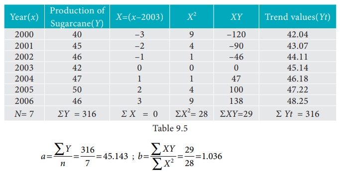
Therefore, the required equation of the straight-line trend is given by
Y = a+bX;
Y = 45.143 + 1.036 (x-2003)
The trend values can be obtained by
When X = 2000, Yt = 45.143 + 1.036(2000–2003) = 42.035
When X = 2001, Yt = 45.143 + 1.036(2001–2003) = 43.071,
similarly, other values can be obtained.
Q6) Given below are the data relating to the sales of a product in a district.
Fit a straight-line trend by the method of least squares and tabulate the trend values.

A6)
Computation of trend values by the method of least squares.
In case of EVEN number of years, let us consider
 similarly other values can be obtained.
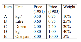
Q7) Construct the cost of living index for the year 1982 (Base 1980 = 100).
A7)
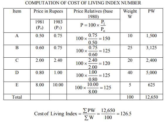
Q8) Calculate the price indices from the following data by applying (1) Laspeyre’s method (2) Paasche’s method and (3) Fisher ideal number by taking 2010 as the base year.
Commodity | 2010 | 2011 | ||
PO | QO | P1 | Q1 | |
A | 20 | 10 | 25 | 13 |
B | 50 | 8 | 60 | 7 |
C | 35 | 7 | 40 | 6 |
D | 25 | 5 | 35 | 4 |
A8)
Commodity | 2010 | 2011 |
|
|
|
| ||
PO | QO | P1 | Q1 | Poqo | P1qo | Poq1 | P1q1 | |
A | 20 | 10 | 25 | 13 | 200 | 250 | 260 | 325 |
B | 50 | 8 | 60 | 7 | 400 | 480 | 350 | 420 |
C | 35 | 7 | 40 | 6 | 245 | 280 | 210 | 240 |
D | 25 | 5 | 35 | 4 | 125 | 175 | 100 | 140 |
|
|
|
|
| 970 | 1185 | 920 | 1125 |
a) Laspeyre’s formula
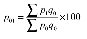
P 01 = (1185/970)*100 = 122.16
b) Paasche’s formula
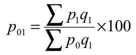
P 01 = (1125/920)*100 = 122.28
c) Fisher’s ideal formula
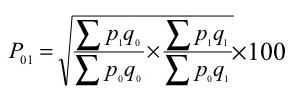
 P 01 = √ = ((1185/970) + (1125/920)) *100 = 120.55
Q9) Calculate the Dorbish and Bowley’s price index number for the following data taking 2014 as base year.
Item | 2010 | 2011 | ||
PO | QO | P1 | Q1 | |
Oil | 80 | 3 | 100 | 4 |
Pulses | 35 | 2 | 45 | 3 |
Sugar | 25 | 2 | 30 | 3 |
Rice | 50 | 30 | 54 | 35 |
A9)
Item | 2010 | 2011 |
|
|
|
| ||
PO | QO | P1 | Q1 | Poqo | P1qo | Poq1 | P1q1 | |
Oil | 80 | 3 | 100 | 4 | 240 | 300 | 320 | 400 |
Pulses | 35 | 2 | 45 | 3 | 70 | 90 | 105 | 135 |
Sugar | 25 | 2 | 30 | 3 | 50 | 60 | 75 | 90 |
Rice | 50 | 30 | 54 | 35 | 1500 | 1620 | 1750 | 1890 |
|
|
|
|
| 1860 | 2070 | 2250 | 2515 |
Dorbish and Bowley’s formula
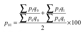
 P 01 = ((2070/1860) + (2515/2250)) *100 = 111.38
2
Q10) Calculate a suitable price index from the following data
Commodity | Quantity | Price | |
|
| 2007 | 2010 |
X | 25 | 3 | 4 |
Y | 12 | 5 | 7 |
Z | 10 | 6 | 5 |
A10)
Commodity | Q | P0 | P1 | P0Q | P1Q |
X | 25 | 3 | 4 | 75 | 100 |
Y | 12 | 5 | 7 | 60 | 84 |
Z | 10 | 6 | 5 | 60 | 50 |
|
|
|
| 195 | 234 |
Kelly price index

= 235/195*100 = 120