Unit 3
Supply and Production Decisions
Q1) Define production function? (5 marks)
A1)
Meaning of production
The term ‘production’ is very important and broader concept in economics. To meet the daily demand of a consumer production is essential part. Production is a process by which various inputs are combined and transformed into output of goods and services, for which there is a demand in the market. In other words, Production is a process of combining various material inputs and immaterial inputs in order to make something for consumption. The essences of production are the creation of utilities and the transformation of inputs or resources into output. Inputs are the resources used in the production of goods and services the important resources or input in production are land, labour, capital, and entrepreneur. Production process creates economic well-being into the nation. Thus, production is a process which creates utility and value in exchange.
The theory of production function is concern with the problem in the production process in a certain level of output. It analyses the relation between cost and output and help the firm to determine its profit. All firms that aims at maximising their profit must make their decision regarding production on the bases of the following three decision:
a. How much output to produce and supply in the market?
b. How to produce the product, i.e. which technique of production or combination of production to used have to be decided?
c. How much quantity of input is demanded to produce the output of the product?
Thus, the above three decisions are interrelated and have to be taken by the firm during the production process.
Production function
To have clear knowledge about production and cost it’s mandatory to know the basics of production functions and understand the fundamentals in mathematical terms. We break down short-term and long-term production functions supported variable and glued factors.
What is the production function?
The functional relationship between the physical input (or factor of production) and therefore the output is named a production function. It assumed the input as an explanatory or independent variable and the output as a dependent variable. Mathematically, you can write this as:
Q=f(L,K)
Where"Q"represents the output,"L"and"K" are the inputs, respectively, labour and capital (such as machinery). Note that there may be many other factors, but we are assuming a two-factor input here. Production functions are defined differently in the short term and in the long term. This distinction is crucial in microeconomics. This distinction is based on the nature of the factor input.
Inputs that change directly with the output are called variable factors. These are factors that can change. Fluctuating factors exist both in the short term and in the long term. Examples of variable factors include daily labour and raw materials.
On the other hand, factors that cannot change or change as the output changes are called fixed factors. These factors are usually characteristic only for a short or short period of time. There are no fixed factors in the long term.
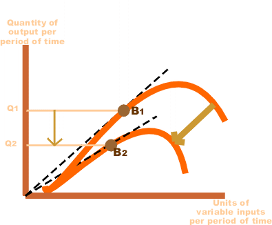
Therefore, two production functions can be defined: short-term and long-term. A short-term production function defines the connection between one variable factor (keeping all other factors fixed) and therefore the output. The law of regression to factors explains such a production function.
For example, suppose that a company has 20 units of Labour and 6 acres of land, and initially uses only Labour units (variable coefficients) for that land (fixed coefficients). Thus, the ratio of land and labour is 6: 1. Now, if the company chooses to adopt 2 labour units, then the ratio of land to Labour will be 3: 1 (6: 2).
Here, all factors change in the same proportion. The law used to explain this is called the law of return to scale. It measures how much of the output changes when the input changes proportionally.
Q2) Define long run production function? (5 marks)
A2)
The functional relationship between the physical input (or factor of production) and therefore the output is named a production function. It assumed the input as an explanatory or independent variable and the output as a dependent variable. Mathematically, you can write this as:
Q=f(L,K)
Where"Q"represents the output,"L"and"K" are the inputs, respectively, labour and capital (such as machinery). Note that there may be many other factors, but we are assuming a two-factor input here. Production functions are defined differently in the short term and in the long term. This distinction is crucial in microeconomics. This distinction is based on the nature of the factor input.
Inputs that change directly with the output are called variable factors. These are factors that can change. Fluctuating factors exist both in the short term and in the long term. Examples of variable factors include daily labour and raw materials.
On the other hand, factors that cannot change or change as the output changes are called fixed factors. These factors are usually characteristic only for a short or short period of time. There are no fixed factors in the long term.
Therefore, two production functions can be defined: short-term and long-term. A short-term production function defines the connection between one variable factor (keeping all other factors fixed) and therefore the output. The law of regression to factors explains such a production function.
Long run production function: The long run production function is defined as the period of time in which all factors of production are variable. In the long run there is no distinction between the fixed or variable factor as all factors in the long run are variable.
The production function can also be classified on the basis of factor proportion i.e. a) Fixed proportion production function and b) Variable proportion production function.
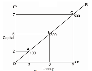
- Fixed proportion production function: The fixed proportion production function, also known as a Leontief Production Function which implies the fixed factors of production function such as land, labour, raw materials are used to produce a fixed quantity of an output and these factors of production function cannot be substituted for the other factors. In other words, in such factors of production function fixed quantity of inputs is used to produce the fixed quantity of output. All factors of production are fixed and cannot be substituted for one another. The concept of fixed proportion production function can be further expained with the help of a Diagram as shown below

Q3) Explain types of production function? (5 marks)
A3)
What is the production function?
The functional relationship between the physical input (or factor of production) and therefore the output is named a production function. It assumed the input as an explanatory or independent variable and the output as a dependent variable. Mathematically, you can write this as:
Q=f(L,K)
Where"Q"represents the output,"L"and"K" are the inputs, respectively, labour and capital (such as machinery). Note that there may be many other factors, but we are assuming a two-factor input here. Production functions are defined differently in the short term and in the long term. This distinction is crucial in microeconomics. This distinction is based on the nature of the factor input.
Inputs that change directly with the output are called variable factors. These are factors that can change. Fluctuating factors exist both in the short term and in the long term. Examples of variable factors include daily labour and raw materials.
On the other hand, factors that cannot change or change as the output changes are called fixed factors. These factors are usually characteristic only for a short or short period of time. There are no fixed factors in the long term.
Therefore, two production functions can be defined: short-term and long-term. A short-term production function defines the connection between one variable factor (keeping all other factors fixed) and therefore the output. The law of regression to factors explains such a production function.
For example, suppose that a company has 20 units of Labour and 6 acres of land, and initially uses only Labour units (variable coefficients) for that land (fixed coefficients). Thus, the ratio of land and labour is 6: 1. Now, if the company chooses to adopt 2 labour units, then the ratio of land to Labour will be 3: 1 (6: 2).
Here, all factors change in the same proportion. The law used to explain this is called the law of return to scale. It measures how much of the output changes when the input changes proportionally.

Types of production function
Short run production function
The short run is defined as the period during which at least one of the input is fixed. According to the following short-run production function, labour is the only variable factor input while the rest of the inputs are regarded as fixed. In other words, the short run is a period in which the firm can adjust production by changing variable factors such as materials and labour but cannot change fixed factors such as land, capital, etc. Thus, in short-run some factors are fixed and some are variable.
Long run production function: The long run production function is defined as the period of time in which all factors of production are variable. In the long run there is no distinction between the fixed or variable factor as all factors in the long run are variable.
The production function can also be classified on the basis of factor proportion i.e. a) Fixed proportion production function and b) Variable proportion production function.
- Fixed proportion production function: The fixed proportion production function, also known as a Leontief Production Function which implies the fixed factors of production function such as land, labour, raw materials are used to produce a fixed quantity of an output and these factors of production function cannot be substituted for the other factors. In other words, in such factors of production function fixed quantity of inputs is used to produce the fixed quantity of output. All factors of production are fixed and cannot be substituted for one another. The concept of fixed proportion production function can be further expained with the help of a Diagram as shown below
B. Variable proportion production function: The variable proportion production function supposes that the ratio in which the factors of production such as labour and capital are used in a variable proportion. Also, the different combinations of factors can be used to produce the given quantity, thus, one factor can be substituted for the other factor. In the case of variable proportion production function, the technical Coefficient of production function is variable, i.e. the important quantity of output can be achieved through the combination of different quantities of factors of production, such as these factors can be varied by substituting one factors to the other/ factors in its place. The concept of variable proportion production function can be further explained from an isoquant curve, as shown in the Diagram below:
Q4) Define isoquant? (5 marks)
A4)
The term “iso-quants” is derived from Greek word iso means “equal” and quants means “quantity”. Thus, iso-quant means equal quantity. An iso-quant is also known as iso-production curve, iso-indifference, equal production curve by various economists. The isoquants have its properties which are similar to those generally assumed for indifference curve theory of the theory of consumer’s behaviour analysis. Iso-quant is defined as “a locus of all the combination of two factors of production that yields that yield the same level of output.”
Thus, an iso-quant is a combination of any two factor inputs that represents and produce the same level of output. Any two combinations of input factors e.g. Labour and capital are used in which one factor is increased by decreasing the other factor of input to maintain the same level of production.
Iso-quant can be explained with the schedule and graph given below:
Factor combinations to produce a given level of output
Factor combination | Labour | Capital | Output |
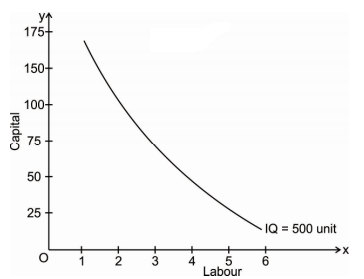
A | 1 | 150 | 500 |
B | 2 | 100 | 500 |
C | 3 | 75 | 500 |
D | 4 | 50 | 500 |
E | 5 | 25 | 500 |
The above table shows the five combination of inputs i.e. Labour and Factor unit which yield the same level of output of 500 units. Which says any point on the iso-quant will give the same level of output. To show this we draw the iso-quant drawn below:
Iso-quant map:
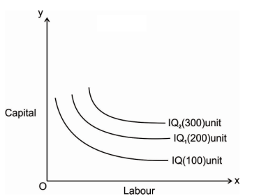
An iso-quant map represents a set of iso-quant curves shows the combination of input factor at the various level of output. A higher level of iso-quant represents the higher level of output. Thus, in simple word, iso-quant map is a family of iso-quant representing the various iso-quant curve at a particular level of output. The iso-quant map can be represented with the diagram given below:
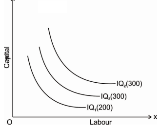
The fig above shows the various iso-quants representing the various level of output at different combination of input factors. IQ1 , IQ2 and IQ3 shows the iso-quant which produces 100,200 and 300 units of output respectively with the various combination of input factors which provides the same level of output at different level of Iso-quant.as we had said higher the Iso-quant represents higher the value of output.
Q5) Define ridge lines? (5 marks)
A5)
The ridge lines are the locus of points of an iso-quants where the marginal product of factors is zero. An isoquant is ovalshaped as shown in diagram but its area of rational operation lies between the ridge lines. The firm will produce only in those segments of isoquants which are convex to the origin and lie between the ridge lines. The ridge lines are the locus of points of isoquants where the marginal products (MP) of factors are zero. The upper ridge line implies zero MP of capital and the lower ridge line implies zero MP of labour. Production techniques are only efficient inside the ridge lines. The marginal products of factors are negative and the methods of production are inefficient outside the ridge lines. The ridge lines can be explained through the help of following diagram:
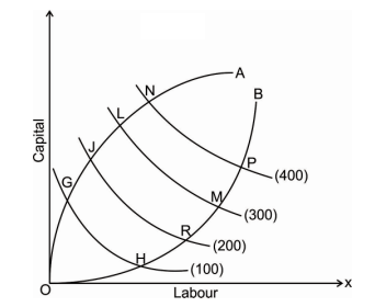
In the above Diagram curves ОA and OB are the ridge lines on the oval-shaped iso-quants and in between these lines on points G, J, L and N and H, К, M and P economically feasible units of capital and labour can be employed to produce 100, 200, 300 and 400 units of the product.
For example, ОТ units of labour and ST units of the capital can produce 100 units of the product, but the same output can be obtained by using the same quantity of labour ОТ and less quantity of capital VT. Thus, only an unwise producer will produce in the dotted region of the isoquant 100. The dotted segments of isoquants form the uneconomic regions of production because they require an increase in the use of both factors with no corresponding in-crease in output. If points G, J, L, N, H, К, M and P are connected with the lines OA and OB, they are the ridge lines. On both sides of the ridge lines, it is uneconomic for the firm to produce while it is economically feasible to produce inside the ridge lines.
Q6) Explain the law of variable proportion? (8 marks)
A6)
Law of variable proportions
The law of variable proportion states that keeping all other factors fixed, when the quantity of one factor increased, the marginal product of that factor will eventually decline. This means that upto the use of a certain amount of variable factor, marginal product of the factor may increase and after a certain stage it starts diminishing. When the variable factor becomes relatively abundant, the marginal product may become negative.
Definition
“As the proportion of the factor in a combination of factors is increased after a point, first the marginal and then the average product of that factor will diminish.” Benham
Assumption
The following assumption of law of variable proportion-
- The state of technology is assumed to be constant.
- Fixed amount of other factors.
- The law is based upon the possibility of varying the proportions in which the various factors can be combined to produce a product.
Illustration of the Law:
The law of variable proportion is explained in the below given table and figure. Assume that a there is a given fixed amount of land, in which more labour (variable factor) is used to produce agricultural product.
Units of labour | Total product | Marginal product | Average product |
1 | 2 | 2 | 2 |
2 | 6 | 4 | 3 |
3 | 12 | 6 | 4 |
4 | 16 | 4 | 4 |
5 | 18 | 2 | 3.6 |
6 | 18 | 0 | 3 |
7 | 14 | -4 | 2 |
8 | 8 | -6 | 1 |
In the above table we can observe that upto the use of 3 units of labour, total product increases at an increasing rate. But after the third unit total product increases at a diminishing rate.
A marginal product is the incremental change in total product as a result of increasing the variable factor i.e labour. We can see from the table, marginal product of labour initially rises and beyond the use of third unit it starts diminishing. The use of 6 units does not add anything in the production. Thus marginal product of labour fallen to zero. After the 6 unit, total product decreases and marginal product becomes negative.
Average product is derived by dividing total product by the quantity of variable unit. Till the 3 unit of labour, average product increases. Whereas after the 3 unit, average product is falling throughout.
Three Stages of the Law of Variable Proportions:
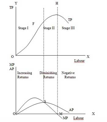
The stages are discussed in the below figure where labour is measured on the X-axis and output on the Y-axis.
Stage 1. Stage of Increasing Returns:
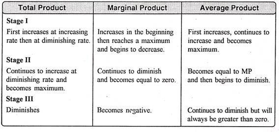
In this stage, total product increases at an increasing rate till point F..ie the curve TP concave upwards upto point F which means marginal product of labour rises. Because efficiency of fixed factor increases with the increase in variable facto labour. After point F, the total product starts increasing at a diminishing rate. Looking at the next figure, marginal product of labour is maximum, after which it diminishes. This stage is called the stage of increasing returns because the average product of the variable factor labour increases throughout this stage. This stage ends at the point where the average product curve reaches its highest point.
Stage 2. Stage of Diminishing Returns:
The stage 2 ends, when the total product increases at a diminishing rate until it reaches it maximum point H. In this stage both marginal product and average product are diminishing but remain positive. Because fixed factor land becomes inadequate with the increase in the quantity of variable factor labour. At point M marginal product is zero which corresponds to the maximum point H of the total product curve.
Stage 3. Stage of Negative Returns:
In stage 3, with the increase in variable factor labour, the total product decline. Therefore the TP curve slopes downward. As a result, marginal product of labour is negative and MP cure falls below x axis. In this case fixed factor land becomes too much inadequate to the increase in variable factor labour.
Q7) Explain the law of returns to scale? (5 marks)
A7)
Laws of Returns to scale
In long run, no factors are fixed. Return of scale refers to proportionate change in productivity from proportionate change in all the inputs.
Definition:
“The term returns to scale refers to the changes in output as all factors change by the same proportion.” Koutsoyiannis
“Returns to scale relates to the behaviour of total output as all inputs are varied and is a long run concept”. Leibhafsky
Types of return of scale-
1. Increasing return of scale.
2. Constant return of scale.
3. Diminishing return of scale.
Explanation
- Increasing return of scale
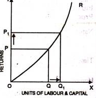
a) When proportionate increase in factors of production leads to higher proportionate increase in production refers to increasing return of scale.
b) In the below figure, x axis represent increase in labour and capital while Y axis represent increase in output. When labour and capital increases from Q to Q1, output also increases from P to P1 which is higher than the change in factors of production ie labour and capital
2. Diminishing return of scale
a) Diminishing return refers to percentage increase in factors of proportion leads to smaller proportion increase in the output
b) For instance, 30% increase in variable input (labour and capital) result in 10% increase in output.
c) In the below diagram, x axis refers increase in labour and capital while Y axis refers increase in output. Percentage increase in labour and capital from Q to Q1 results in less percentage change in output from P to P1

3. Constant return of scale
a) Constant return of scale refers to output increases in same proportion in which factors of production (labour and capital) increases.
b) Internal and external economies is equal to internal and external diseconomies
c) This is known as homogenous production function
d) In the below figure, x axis refers increase in labour and capital while Y axis refers increase in output. Increase in labour and capital from Q to Q1 is equal to the increases in output from P To P1

Q8) What is isoquant? Discuss its properties in detail? (8 marks)
A8)
Isoquants
The term “iso-quants” is derived from Greek word iso means “equal” and quants means “quantity”. Thus, iso-quant means equal quantity. An iso-quant is also known as iso-production curve, iso-indifference, equal production curve by various economists. The isoquants have its properties which are similar to those generally assumed for indifference curve theory of the theory of consumer’s behaviour analysis. Iso-quant is defined as “a locus of all the combination of two factors of production that yields that yield the same level of output.”
Thus, an iso-quant is a combination of any two factor inputs that represents and produce the same level of output. Any two combinations of input factors e.g. Labour and capital are used in which one factor is increased by decreasing the other factor of input to maintain the same level of production.
Iso-quant can be explained with the schedule and graph given below:
Factor combinations to produce a given level of output
Factor combination | Labour | Capital | Output |
A | 1 | 150 | 500 |
B | 2 | 100 | 500 |
C | 3 | 75 | 500 |
D | 4 | 50 | 500 |
E | 5 | 25 | 500 |
The above table shows the five combination of inputs i.e. Labour and Factor unit which yield the same level of output of 500 units. Which says any point on the iso-quant will give the same level of output. To show this we draw the iso-quant drawn below:

Iso-quant map:
An iso-quant map represents a set of iso-quant curves shows the combination of input factor at the various level of output. A higher level of iso-quant represents the higher level of output. Thus, in simple word, iso-quant map is a family of iso-quant representing the various iso-quant curve at a particular level of output. The iso-quant map can be represented with the diagram given below:

The fig above shows the various iso-quants representing the various level of output at different combination of input factors. IQ1 , IQ2 and IQ3 shows the iso-quant which produces 100,200 and 300 units of output respectively with the various combination of input factors which provides the same level of output at different level of Iso-quant.as we had said higher the Iso-quant represents higher the value of output.
Properties
- Iso-quant curve slopes downwards: The iso-quant curve slopes downwards from left to right i.e. it has a negative slope. The slope is downward because it operates under law of MRTS, when we increase labour as a factor, we have to decrease capital factor to produce a same level of output. The downward sloping iso-quant curve can be explaining the help of following Diagram
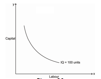
Thus, the iso-quant can be downward sloping from left to right. There can’t be an upward sloping iso-quant curve because it shows that a given product can be produce by using less of both the input factor. Similarly, an iso-quant cannot be horizontal or vertical because it also doesn’t represent the equilibrium position of a firm. Only the downward sloping supply curve represents the characteristics of iso-quant.
2. Iso-quant are convex to the origin: As we had discussed in the above property that the iso-quant curve is downward sloping and it has a negative slope and it operates under law of Marginal rate of Technical Substitution (MRTS). It says that it equals the ratio of the marginal product if labour and marginal product of capital i.e. one factor is given up to get one additional unit of other factor to produce the same of output which creates a convexity of iso-quant curve.
Thus, the slope of iso-quant can be represented by,

The above equation represents ratio of change in capital and labour should be equal to the ratio of the marginal rate of technical substitution of labour and capital which is equal to the ratio of marginal product of labour and capital.
The convexity of iso-quant means that as we move down the curve less and less of capital given up for an additional unit of labour so to produce the same level of output. The convexity of isoquant can be observed from the diagram Given below
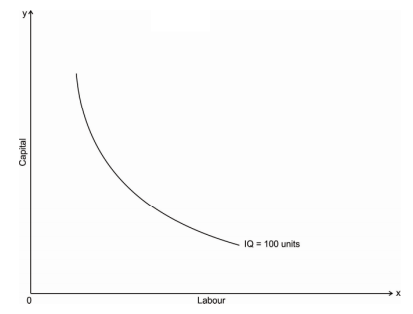
Thus, the iso-quant can be convex to the origin but not the concave because it would mean that MRTS will increase instead of decreasing i.e. labour will increase at a constant rate the amount of capital given up will goes on increasing
3. Iso-quants do not intersect: The properties of iso-quants say that two iso-quant will never intersect each other. To explain this, we will take a help of following Diagram
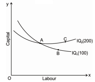
The above fig represents two different iso-quant IQ1and IQ2, where it represents the level of output 100 and 200 units respectively. Point a represents 100 units of output on IQ1 and point c represents 200 units of output on IQ2. The point b shows the intersection of both the iso-quants where is logically not possible to identify the level of output.
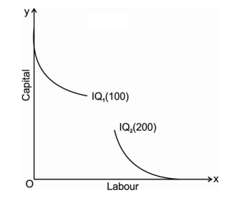
4. Iso-quant cannot touch either of the axis: An iso-quant cannot only touch x axis or y axis or any either axis because it will represent that the iso-quant only produce goods by using one factors of production either by using only capital or only labour which is practically not possible and which is unrealistic.
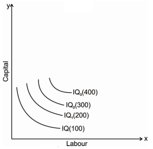
5. Higher the iso-quant higher the level of production: if there is a multiple iso-quant showing different level of production in one diagram. Where the higher the iso-quant i.e. the iso-quant far from the origin indicates higher level of output and the iso-quant close to the origin indicates lower level of output.
Q9) Write a short note on: a. Ridge lines b. Expansion path ? (5 marks)
A9)
Ridge lines
The ridge lines are the locus of points of an iso-quants where the marginal product of factors is zero. An isoquant is ovalshaped as shown in diagram but its area of rational operation lies between the ridge lines. The firm will produce only in those segments of isoquants which are convex to the origin and lie between the ridge lines. The ridge lines are the locus of points of isoquants where the marginal products (MP) of factors are zero. The upper ridge line implies zero MP of capital and the lower ridge line implies zero MP of labour. Production techniques are only efficient inside the ridge lines. The marginal products of factors are negative and the methods of production are inefficient outside the ridge lines. The ridge lines can be explained through the help of following diagram:

In the above Diagram curves ОA and OB are the ridge lines on the oval-shaped iso-quants and in between these lines on points G, J, L and N and H, К, M and P economically feasible units of capital and labour can be employed to produce 100, 200, 300 and 400 units of the product.
For example, ОТ units of labour and ST units of the capital can produce 100 units of the product, but the same output can be obtained by using the same quantity of labour ОТ and less quantity of capital VT. Thus, only an unwise producer will produce in the dotted region of the isoquant 100. The dotted segments of isoquants form the uneconomic regions of production because they require an increase in the use of both factors with no corresponding in-crease in output. If points G, J, L, N, H, К, M and P are connected with the lines OA and OB, they are the ridge lines. On both sides of the ridge lines, it is uneconomic for the firm to produce while it is economically feasible to produce inside the ridge lines.
Expansion path
In economics, an expansion path is a line connecting optimal input combinations as the scale of production expands. A producer seeking to produce the most units of a product in the cheapest possible way to increase production along the expansion path.
Definition
Economist Alfred Stonier and Douglas Hague defined expansion path as,” that line which reflects least cost method of producing different levels of output, when factor prices remains constant”.
Assumption
a) There are two factors of production, labour and capital, which are variable.
b) All units of labour and capital are homogeneous.
c) The price of labour is constant.
d) The price of capital is constant.
e) The firm increases its total outlay in order to expand its output.
In order to maximise profits, the firm combines labour and capital in such a way that the ratio of their MP is equal to the ratio of their prices

This occurs at a point of tangency between an isocost line and an isoquant curve.

In the above figure, the different isoquant lines areC1L1,C2L2,C3L3. Keeping the prices of factors constant, the different isoquant lines are shown parallel to each other. There are three isoquants ie 100, 200, 300 representing successively higher level of output.
At point P, the firm is at equilibrium, where the isoquant 100 is tangent to its corresponding isoquant line C1L1. Similarly the firm is equilibrium at point Q and R, where the isoquant 200 and 300 is tangent to its corresponding isoquant line C2L2 and C3L3. Each point of tangency implies optimum combination of capital and labour that produces optimum level of output. The line OS joining the equilibrium point P,Q,R from the origin is the expansion path of the firm.
Q10) Explain the internal and external economies of scale? (8 marks)
A10)
Economies of scale are the factors which reduces the production cost as the volume of output increases. This means firm produces more output, then marginal cost of production decreases.
Economies of scale is divided into internal and external
Internal economies of scale – internal economies are caused by factors within the firm. It measures the company efficiency of production. The company focus on improving the output to reduce the product average cost.
Six different types of internal economies of scale: (1) technical, (2) managerial, (3) marketing, (4) financial, (5) commercial, and (6) network economies of scale.
- Technical economies of scale – This can be achieved through improvements and optimizations within the production process. When the output increases, the firm will invest more in efficient equipment and optimise operation based on experience. Efficient machinery result in producing output at lower cost.
2. Managerial economies of scale - The employment of specialised workforce result in managerial economies of scale. As the organisation grow, they hire more expert staff and create a specialised business unit. The firm efficiency is increased by employing specialist, accountants, human resource, etc which will result in reducing the cost of production and increase revenue.
3. Marketing economies of scale – Marketing economies of scale is the ability to spread advertising and marketing budget over an increasing output. As the production increases the firm can fix marketing expenses, which will reduce the per unit cost of production. Better advertisement result in reaching larger audience and increase the sale of the firm.
4. Financial economies of scale – Access of financial and capital market result in financial economies of scale. Large firms find easier and cheaper to raise funds. As the firm grow, it is considered to be more credit worthy. They can easily raise fund from banks, stock markets.
5. Commercial economies of scale – Reduction in price due to discounts or bargaining power result in commercial economies of scale. Larger firms can buy goods and services in larger quantities. Thus they get larger discount and can bargin to negotiate lower prices. This means they pay less for each item purchases.
6. Network economies of scale - When the marginal costs of adding additional customers are extremely low result in network economies of scale. This means larger firm can support large numbers of new customers with their existing infrastructure can substantially increase profitability as they grow.
External economies of scale – external economies of scale are caused by changes outside the firm but within the industry. The factors affect the whole industry. Four different types of external economies of scale: (1) infrastructure, (2) supplier, (3) innovation, and (4) lobbying economies of scale.
- Infrastructure - Public infrastructure that is put in place to benefit a specific industry result in infrastructure economies of scale. When many firms of same industry are located nearby, the government will expand infrastructure such as roads, transport, etc to meet their needs.
2. Specialization economies of scale – When suppliers and workers focus on a particular industry due to its size result in specialization economies of scale. When company within the industry increases its size and numbers, suppliers focus in that particular industry. Similarly, similarly workers find job in those industry which is growing in size.
3. Innovation economies of scale – Increases public and private research result in innovation economies of scale. Industries have significant impact on the society result in growing public interest. This allows them to collaborate with research facilities and university to improve their products and processes
4. Lobbying economies of scale - Lobbying economies of scale arise from an increase in bargaining power as industries become more significant. The government is ready to compromise as these industry provide a lot of jobs and pay a significant amount of taxes.
Q11) Explain the internal and external economies of scale? (8 marks)
A11)
Uneconomics of scale occurs when the long-term average cost of an organization increases. It can occur when the tissue becomes excessively large. In other words, uneconomics of Scale Causes larger org-anizations to produce goods and services at increased costs.
There are two types of scale diseconomies: internal diseconomies and external diseconomies, which are discussed as follows:
i.Internal uneconomics of the scale:
See uneconomical raising the cost of production in the organization. The main factors affecting the cost of production of the organization include the lack of determination, supervision and technical difficulties.
Ii.External uneconomics of the scale:
See uneconomical to limit the expansion of an organization or industry. Factors acting as restraints on expansion include increased production costs, a shortage of raw materials and a decline in the supply of skilled workers.
There are several causes of diseconomics of scale.
Some of the causes that lead to uneconomics of scale are:
i.Act as the main reason for diseconomics of scale.
If the organization's production goals and objectives are not properly communicated to employees in the organization, they can lead to overproduction or production. This can lead to diseconomics of scale.
Separately, if the communication process in the organization is not strong, then the employee will not get enough feedback. As a result, there will be less face-to-face interaction between employees, which will affect the production process.
Ii.Lack of motivation:
This leads to a decrease in productivity levels. For large organizations, workers may feel isolated and less motivated because they are less valued for their work. Because of poor communication networks, it is difficult for employers to interact with employees and build a sense of attributes. This leads to a decrease in the productivity level of output due to lack of motivation. This further leads to an increase in the cost of the organization.
Iii.Loss of control:
It serves as the main problem of large organizations. Monitoring and controlling the work of all employees in a large organization becomes impossible and expensive. It is difficult to make sure that all employees of the organization are working towards the same goal. It becomes difficult for managers to direct the sub-coordinates of large organizations.
Iv.Cannibalism:
It means a situation where an organization is facing competition from its products. While smaller organizations face competition from the products of other organizations, larger organizations find their products compete with each other.
Q12) Write a short note on: Economies of scope? (5 marks)
A12)
Economies of scope refer to a situation where in the long-run a firm tries to reduces average and marginal cost of production by producing large varieties of output. In other words, economies of means a firm produces multiple products instead of producing one single product to increases his scope of output by using the same equipment’s and machine as a result of this average cost decreases.
Economies of scope is different from economies of scale, in that where the former means producing a variety of different products or multiple of product together to reduce costs while the latter means producing more of the same product in order to reduce the costs by increasing the efficiency in production.
Economies of scope can arise from the co-production relationships between the final products or the actual products. In economic terms these goods are complements in production. This is when the production of one good automatically produces another good as a by-product or a kind of side-effect in the production process. Sometimes one product might be a by-product of another, but have value for use by the producer or for sale. Finding a productive use or market for the co-products can reduce costs or increase revenue.
For example, dairy farmers separate milk into whey and curds, with the curds going on to become cheese. In the process they also end up with a lot of whey, which they can use as a high protein feed for livestock to reduce their feed costs or sell as a nutritional product to fitness enthusiasts and weightlifters for additional revenue. Another example of this is the black liquor produced by the processing of wood into paper pulp. Instead of being just a waste product that might be costly to dispose of, black liquor is burned as an energy source to fuel and heat the plant, saving money on other fuels, or can even be processed into more advanced bio-fuels for use on-site or for sale. Producing and using the black liquor saves costs on producing the paper.
For example, a shoe manufacture produces men’s and women’s sneakers. If he adds a children’s line of sneakers would increase economies of scope because to make a new line of products he can use the same production equipment, supplies, storage, and distribution channels. Thus the cost of production will be reduced.
In such case due to the production of complemetary goods and services the long run average and marginal cost of the company decreases.
Q13) Explain causes of diseconomies of scale? 5 marks
A13) Uneconomics of scale occurs when the long-term average cost of an organization increases. It can occur when the tissue becomes excessively large. In other words, uneconomics of Scale Causes larger org-anizations to produce goods and services at increased costs.
There are two types of scale diseconomies: internal diseconomies and external diseconomies, which are discussed as follows:
i.Internal uneconomics of the scale:
See uneconomical raising the cost of production in the organization. The main factors affecting the cost of production of the organization include the lack of determination, supervision and technical difficulties.
Ii.External uneconomics of the scale:
See uneconomical to limit the expansion of an organization or industry. Factors acting as restraints on expansion include increased production costs, a shortage of raw materials and a decline in the supply of skilled workers.
There are several causes of diseconomics of scale.
Some of the causes that lead to uneconomics of scale are:
i.Act as the main reason for diseconomics of scale.
If the organization's production goals and objectives are not properly communicated to employees in the organization, they can lead to overproduction or production. This can lead to diseconomics of scale.
Separately, if the communication process in the organization is not strong, then the employee will not get enough feedback. As a result, there will be less face-to-face interaction between employees, which will affect the production process.
Ii.Lack of motivation:
This leads to a decrease in productivity levels. For large organizations, workers may feel isolated and less motivated because they are less valued for their work. Because of poor communication networks, it is difficult for employers to interact with employees and build a sense of attributes. This leads to a decrease in the productivity level of output due to lack of motivation. This further leads to an increase in the cost of the organization.
Iii.Loss of control:
It serves as the main problem of large organizations. Monitoring and controlling the work of all employees in a large organization becomes impossible and expensive. It is difficult to make sure that all employees of the organization are working towards the same goal. It becomes difficult for managers to direct the sub-coordinates of large organizations.
Iv.Cannibalism:
It means a situation where an organization is facing competition from its products. While smaller organizations face competition from the products of other organizations, larger organizations find their products compete with each other.
Q14) Explain different types of external and internaleconomies of scale ? 5 marks.
A14) Economies of scale are the factors which reduces the production cost as the volume of output increases. This means firm produces more output, then marginal cost of production decreases.
Economies of scale is divided into internal and external-
Internal economies of scale – internal economies are caused by factors within the firm. It measures the company efficiency of production. The company focus on improving the output to reduce the product average cost.
Six different types of internal economies of scale: (1) technical, (2) managerial, (3) marketing, (4) financial, (5) commercial, and (6) network economies of scale.
- Technical economies of scale – This can be achieved through improvements and optimizations within the production process. When the output increases, the firm will invest more in efficient equipment and optimise operation based on experience. Efficient machinery result in producing output at lower cost.
- Managerial economies of scale - The employment of specialised workforce result in managerial economies of scale. As the organisation grow, they hire more expert staff and create a specialised business unit. The firm efficiency is increased by employing specialist, accountants, human resource, etc which will result in reducing the cost of production and increase revenue.
- Marketing economies of scale – Marketing economies of scale is the ability to spread advertising and marketing budget over an increasing output. As the production increases the firm can fix marketing expenses, which will reduce the per unit cost of production. Better advertisement result in reaching larger audience and increase the sale of the firm.
- Financial economies of scale – Access of financial and capital market result in financial economies of scale. Large firms find easier and cheaper to raise funds. As the firm grow, it is considered to be more credit worthy. They can easily raise fund from banks, stock markets.
- Commercial economies of scale – Reduction in price due to discounts or bargaining power result in commercial economies of scale. Larger firms can buy goods and services in larger quantities. Thus they get larger discount and can bargin to negotiate lower prices. This means they pay less for each item purchases.
- Network economies of scale - When the marginal costs of adding additional customers are extremely low result in network economies of scale. This means larger firm can support large numbers of new customers with their existing infrastructure can substantially increase profitability as they grow.
External economies of scale – external economies of scale are caused by changes outside the firm but within the industry. The factors affect the whole industry. Four different types of external economies of scale: (1) infrastructure, (2) supplier, (3) innovation, and (4) lobbying economies of scale.
- Infrastructure - Public infrastructure that is put in place to benefit a specific industry result in infrastructure economies of scale. When many firms of same industry are located nearby, the government will expand infrastructure such as roads, transport, etc to meet their needs.
- Specialization economies of scale – When suppliers and workers focus on a particular industry due to its size result in specialization economies of scale. When company within the industry increases its size and numbers, suppliers focus in that particular industry. Similarly, similarly workers find job in those industry which is growing in size.
- Innovation economies of scale – Increases public and private research result in innovation economies of scale. Industries have significant impact on the society result in growing public interest. This allows them to collaborate with research facilities and university to improve their products and processes
- Lobbying economies of scale - Lobbying economies of scale arise from an increase in bargaining power as industries become more significant. The government is ready to compromise as these industry provide a lot of jobs and pay a significant amount of taxes.
Q15) Explain expansion path and law of return of scale? 5 marks
A15) Laws of Returns to scale
In long run, no factors are fixed. Return of scale refers to proportionate change in productivity from proportionate change in all the inputs.
Definition:
“The term returns to scale refers to the changes in output as all factors change by the same proportion.” Koutsoyiannis
“Returns to scale relates to the behaviour of total output as all inputs are varied and is a long run concept”. Leibhafsky
Types of return of scale
1. Increasing return of scale.
2. Constant return of scale.
3. Diminishing return of scale.
Explanation
- Increasing return of scale
a) When proportionate increase in factors of production leads to higher proportionate increase in production refers to increasing return of scale.
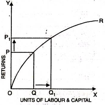
b) In the below figure, x axis represent increase in labour and capital while Y axis represent increase in output. When labour and capital increases from Q to Q1, output also increases from P to P1 which is higher than the change in factors of production ie labour and capital

2. Diminishing return of scale
a) Diminishing return refers to percentage increase in factors of proportion leads to smaller proportion increase in the output.
b) For instance, 30% increase in variable input (labour and capital) result in 10% increase in output.
c) In the below diagram, x axis refers increase in labour and capital while Y axis refers increase in output. Percentage increase in labour and capital from Q to Q1 results in less percentage change in output from P to P1.
3. Constant return of scale
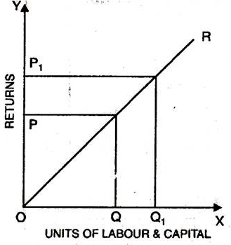
a) Constant return of scale refers to output increases in same proportion in which factors of production (labour and capital) increases.
b) Internal and external economies is equal to internal and external diseconomies.
c) This is known as homogenous production function.
d) In the below figure, x axis refers increase in labour and capital while Y axis refers increase in output. Increase in labour and capital from Q to Q1 is equal to the increases in output from P To P1
Key takeaways –
- Return of scale refers to proportionate change in productivity from proportionate change in all the inputs.
Expansion path
In economics, an expansion path is a line connecting optimal input combinations as the scale of production expands. A producer seeking to produce the most units of a product in the cheapest possible way to increase production along the expansion path.
Definition
Economist Alfred Stonier and Douglas Hague defined expansion path as,” that line which reflects least cost method of producing different levels of output, when factor prices remains constant”.
Assumption
a) There are two factors of production, labour and capital, which are variable.
b) All units of labour and capital are homogeneous,
c) The price of labour is constant,
d) The price of capital is constant,
e) The firm increases its total outlay in order to expand its output.
In order to maximise profits, the firm combines labour and capital in such a way that the ratio of their MP is equal to the ratio of their prices.

This occurs at a point of tangency between an isocost line and an isoquant curve.
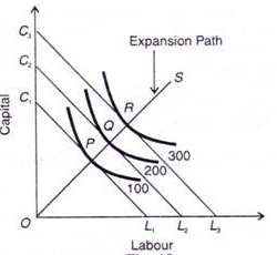
In the above figure, the different isoquant lines areC1L1,C2L2,C3L3. Keeping the prices of factors constant, the different isoquant lines are shown parallel to each other. There are three isoquants ie 100, 200, 300 representing successively higher level of output.
At point P, the firm is at equilibrium, where the isoquant 100 is tangent to its corresponding isoquant line C1L1. Similarly the firm is equilibrium at point Q and R, where the isoquant 200 and 300 is tangent to its corresponding isoquant line C2L2 and C3L3. Each point of tangency implies optimum combination of capital and labour that produces optimum level of output. The line OS joining the equilibrium point P,Q,R from the origin is the expansion path of the firm.