|
|
|
|
|
|
|
|
|
|
|
|
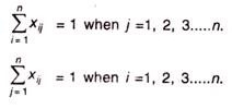
 Be constrained
 If the aggregate supply from all sources is equal to the aggregate demand of all destinations, then x11 of all i and j is said to be a balanced transport problem, otherwise the problem is an imbalanced transport problem is said to be.There may be a solution that can only be implemented if the transportation problem is a balanced problem. Imbalanced issues can be balanced by adding dummy supply centers (rows) or dummy demand centers, depending on your requirements. Q6) Explain Prohibited Transportation Problems, Unique or Multiple Optimal Solutions.A6) Sometimes, there may be situations when a particular route cannot be used for transportation, for example, when road is being constructed, accidents, floods, etc. These problems are known as prohibited transportation problems. These can be solved by two methods:
It is possible that a transportation problem to have multiple optimal solutions. This happens when one or more of the improvement indices are zero in the optimal solution. This means that there is a possibility for designing alternative shipping routes with the same total shipping cost. The alternate optimal solution can be found by shipping the most to this unused square using a stepping-stone path. In the real world, alternate optimal solutions help with better management and greater flexibility in selecting and using resources.
Consider the following transportation problem.Factory | Warehouse | Supply | ||
W1 | W2 | W3 | ||
F1 | 16 | ∞ | 12 | 200 |
F2 | 14 | 8 | 18 | 160 |
F3 | 26 | ∞ | 16 | 90 |
Demand | 180 | 120 | 150 | 450 |
Factory | Warehouse | Supply | ||
W1 | W2 | W3 | ||
F1 |
| ∞ |
| 200 |
F2 |
|
| 18 | 160 |
F3 |
| ∞ | 16 | 90 |
Demand | 180 | 120 | 150 | 450 |
|
| DESTINATIONS |
|
| SUPPLY |
|
| 1 | 2 | 3 |
|
| A | 2 | 3 | 1 | 10 |
SOURCE | B | 5 | 4 | 8 | 35 |
| C | 5 | 6 | 8 | 25 |
DEMAND |
| 20 | 25 | 25 |
|
|
|
|
|
|
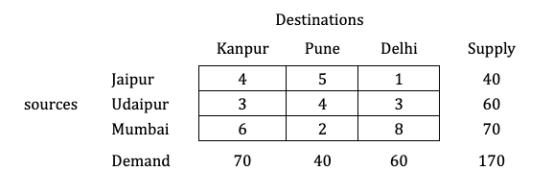
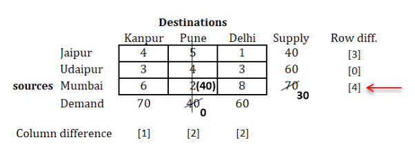
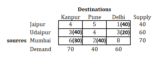
A mobile phone manufacturing company has three branches which are located in three different regions, say Jaipur, Udaipur and Mumbai. The company is supposed to transport mobile phones to three destinations, say Kanpur, Pune and Delhi. The availability from Jaipur, Udaipur and Mumbai is 40, 60 and 70 units respectively. The demand at Kanpur, Pune and Delhi are 70, 40 and 60 respectively. The transportation cost is shown in the matrix below (in Rs). Use the Vogel’s Approximation Method to find a basic feasible solution (BFS).
|
|
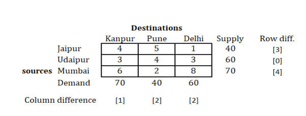
Hence, we find 1 and 4 as the two lowest values in the first row.
Take the difference of these two numbers, i.e. (4−1)=3.
In a similar manner, find out differences for all the rows as shown above.
The same procedure is to be done with columns.
So, for the first column, you will get, (4−3)=1.
Find out difference for all columns as done above.Step 3: Select the row/column with highest difference
|
So we will select that row, and find out the minimum cost in that row.
You will find that, minimum cost is 2.
Now, compare the supply and demand for this row and column respectively.
We find that, we have supply as 70 and demand as 40 for the selected cell.
Compare both and select the minimum of them for the allocation in the cell, as shown below.
Cross out the column whose demand is fulfilled.Step 4: Remove the row/column whose supply or demand is fulfilled and prepare new matrix and repeat the same procedure
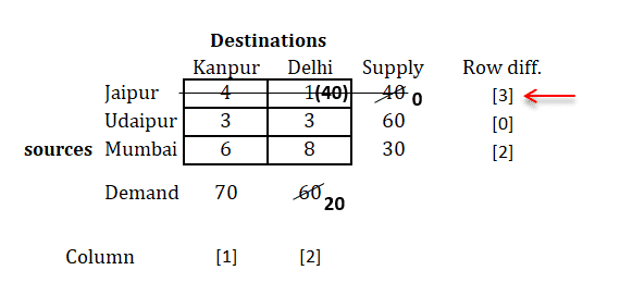
|
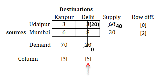
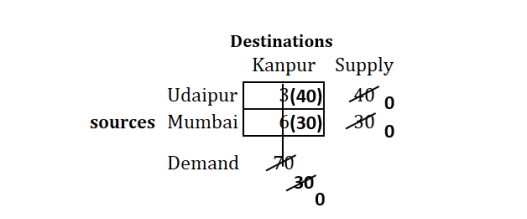
Now, we will repeat the same procedure until we're done with all allocations.
i.e.,
|
|
|
|
|
|
|
|
|
|
|
|
|
|
|
|
|
|
| D1 | D2 | D3 | D4 | Availability |
O1 | 1 | 2 | 1 | 4 | 30 |
O2 | 3 | 3 | 2 | 1 | 50 |
O3 | 4 | 2 | 5 | 9 | 20 |
Requirement | 4 | 40 | 30 | 10 | 100 |
| D1 | D2 | D3 | D4 | Availability | Row Differences |
01 | 1
(20) | 2 | 1
(10) | 4 | 30/10/0 | [0] [0] [1] |
O2 | 3 | 3
(20) | 2
(20) | 1 (10) | 50/40/20/0 | [1] [1] [1] |
03 | 4 | 2
(20) | 5 | 9 | 20/0 | [2] [2] |
Requirement | 20/0 | 40/20/0 | 30/20/0 | 10/0 | 100/100 |
|
Column Differences | [2] [2] | [0] [0] [1] | [1] [1] [1] | [3] |
|
|
|
|
|


