Unit - 3

Transportation problem and its mathematical formulation

Q1) Define transportation problems.

A1)

The transportation algorithms help to minimize the total cost of transporting a homogeneous commodity (product) from supply centres to demand centres. However, it can also be applied to the maximization of total value or utility.

The structure of transportation problem involves a large number of shipping routes from several supply centres to several demand centres. Thus, objective is to determine shipping routes between supply centres and demand centres in order to satisfy the required quantity of goods or services at each destination centre, with available quantity of goods or services at each supply centre at the minimum transportation cost and/ or time.

Q2) Give general Mathematical Model of Transportation Problem.

A2)

Let there be m sources of supply, S1, S2, . . ., Sm having ai (i = 1, 2, . . ., m) units of supply (or capacity), respectively to be transported to n destinations, D1, D2, . . ., Dn with bj ( j = 1, 2, . . ., n) units of demand (or requirement), respectively. Let cij be the cost of shipping one unit of the commodity from source i to destination j. If xij represents number of units shipped from source i to destination j, the problem is to determine the transportation schedule so as to minimize the total transportation cost while satisfying the supply and demand conditions. Mathematically, the transportation problem, in general, may be stated as follows:

Subject to the constraints

And

Q3) What is the simple Formulation of Transportation Problems

A3)

Let a manufacturer of an item has m origin situated at places O1, O2, . . ., Oi, . . ., Om and let there are n destinations at D1, D2, . . . Dj . . . Dn. The aggregate of the capacities of all m origins is assumed to be equal to the aggregate of the requirements of all n destinations. Let Cij be the cost of transporting one unit from origin i to destination j. Let ai be the capacity/availability of items at origin i and bj , the requirement/demand of the destination j.

Then this transportation problem can be expressed in a tabular form as given below-

Origin	Destinations        .  .  . . . . . .	Capacity
. . .   . . .	.  .   . . . . .     .  .   . . . . . . . .       .  .   . . . . . . . .     .  . . . . . .	. . . . .   .
Requirement	.    . . . .   . .	Total

For the existence of a feasible solution to a transportation problem is given as

This equation define that the total requirement equals the total capacity. If it is not so, a dummy origin or destination is created to balance the total capacity and requirement.

Let xij be the number of units to be transported from origin i to destination j and Cij the corresponding cost of transportation. Then the total transportation cost is .

This means that the product of the number of units allocated to each cell with the transportation cost per unit for that cell is calculated and added for all cells. Our objective is to allocate the units in such a way that the total transportation cost is least. The problem can also be stated as a linear programming problem as follows:

We are to minimise the total transportation cost-

Subject to the constraints-

And

For all i = 1,2, ...., m and j = 1,2, ......n.

This problem can be solved by the simplex method but it is very lengthy so that we use an alternative method which is the ‘transportation method’.

Q4) Give steps of North West Corner Rule (NWCR)

A4)

1. Select the North-west (i.e., upper left) corner cell of the table and allocate the maximum possible units between the supply and demand requirements. During allocation, the transportation cost is completely discarded (not taken into consideration).

2. Delete that row or column which has no values (fully exhausted) for supply or demand.

3. Now, with the new reduced table, again select the North-west corner cell and allocate the available values.

4. Repeat steps (2) and (3) until all the supply and demand values are zero.

5. Obtain the initial basic feasible solution.

Q5) Find out the initial feasible solution for transportation cost involved in the problem shown in table:

A5)

As under the process of NWC method, we allocate = 20. Now demand for the first column is satisfied, therefore, eliminate that column.

Proceeding in this way, we observe that

Delete the row if supply is exhausted.

Delete the column if demand is satisfied.

Here, number of retail shops (n) = 4, and

Number of factories (m) = 3

Number of basic variables = m + n – 1 = 3 + 4 – 1 = 6.

Initial basic feasible solution:

20 × 3 + 20 × 5 + 10 × 7 + 40 × 8 + 35 × 2 + 25 × 2 = 670

Q6) Explain Vogel’s Approximation Method (VAM)

A6)

1. For each row of the transportation table, we identify the least and second least costs. We find the difference between these two and display it to the right of that row in a new column formed by extending the table on the right. Likewise, we find such differences for each column and display it below that column in a new row formed for the purpose by extending the table at the bottom. The new column and row formed by extending the table at the right and bottom are labelled as penalty column and penalty row, respectively. If two cells in a row (or column) contain the same least costs then the difference is taken as zero.
2. From amongst these difference values displayed in the penalty column and the penalty row, we select the largest value (largest difference). We, allocate the maximum possible units to the least cost cell in the selected column or row. If a tie occurs amongst the largest differences, the choice may be made for that row or column, which has the least cost. In case there is a tie in such least cost as well, choice may be made from that row or column by which maximum requirements are exhausted. The cell so chosen is allocated the units and the corresponding exhausted row (or column) is removed (or ignored) from further consideration.
3. We compute the column and row differences for the reduced transportation table and repeat the procedure until all column and row totals are exhausted.

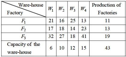
Q7) Find the initial Basic feasible solution of the following transportation problem by Vogel’s apprx. Method.

A7)

Step-1: Here, the total production of the factories and total capacities of the ware-houses being the same i.e. 43, the problem is balanced.

Step-2: Initial Basic Feasible solution- By VAM the difference between the smallest and next to the smallest costs in each row and each column are computed and written within brackets against the respective rows and column of table 1.

From table-1,

Largest difference (10) corresponds to 4th column. In this column, first row corresponds to lowest cost (13). So allocate to (1, 4) box with min (11, 23) ie 11.

The first row is exhausted. The reduced table 1 is written below

From table-2,

Largest difference 18 corresponds to 4th column. In this column first row corresponds to the lowest cost (13). So allocate to (1, 4) box min (4, 13) i.e. 4.

Fourth column is exhausted. The reduced table is written below

From table 3, largest difference (15) corresponds to first column. In this column first row corresponds to the lowest cost (17). So allocate to the (1, 1) box with the min (6, 9) ie 6.

First column of table - 3 is exhausted and the reduced table 4 is written below.

The largest difference (9) occurs at two places. So there is a tie here. Costs on both largest differences are identical choose any one. Allocate (1, 1) box with min (3, 10) i.e. 3.

First row of table-4 is exhausted. The reduced table 4 is written below:

From table 5, largest difference (27) corresponds to first column and is written in the box of first column and first row.

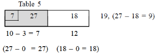
First column of table 5 is exhausted. The reduced table 6 has only one box.

From table 6, minimum of 12 and 12 is 12 and is written in this box.

The initial basic feasible solution is given in the table below-

Q8) What is the mathematical formulation of assignment problems?

A8)

The basic viable solution to the allocation problem cons

Ists of (2n – 1) variables, where the (n – 1) variable is zero and n is that the number of jobs or facilities. Thanks to this high degree of degeneracy, solving problems with normal shipping methods are often a posh and time-consuming task. Therefore, another method springs . it's vital to formulate the matter before proceeding to absolutely the law.

Suppose xjj may be a variable defined as follows:

If the primary job is assigned to the jth machine or facility

0 if the i-th job isn't assigned to the j-th machine or facility.

Therefore,

Here, the matter is made one-to-one, or one job is assigned to at least one facility or machine.

The total allocation cost is

The above definition is often evolved into a mathematical model as follows:

Determine xij> 0 (i, j = 1,2,3… n),

Minimize,

Be constrained

Xij is either 0 or 1.

- indicates the cost of assigning ith job to jth individual or vice versa, Viij = 1 to n.

- indicates whether ith job is assigned to jth person or not.

if ith job is assigned to jth person ‘0’ otherwise.

Q9) Solve the following assignment problem and find the minimum cost.

A9)

Here we will use reduction rules,

Step 1: Row-wise Reduction of the matrix.

Step 2: Column-wise Reduction of the matrix.

Step 3: Assignment of jobs to workers.

Step 4: Calculation of the Minimum total job cost associated with the assignment.

The minimum total cost required to complete the assignment is Rs. 38.

Q10) A company has taken the third floor of a multi-storied building for rent to locate one of its zonal offices. There are five main rooms in this floor to be assigned to five managers. Each room has its own advantages and disadvantages. Some have two cupboards, some are closer to the washrooms or to the canteens, some are of big sizes and are on different floors, etc. Each of the five managers were asked to rank their room preferences amongst the rooms 201, 302, 103, 304 and 205. Their preferences were recorded in a table as indicated below:

Manager                                                                                                          302          302           103          302           201                              103          304           201          205           302      Rooms           304          205            304          304           304                                              201            205         103                                                                       302

Most of the managers did not include all five rooms in the list since they were not satisfied with some of them. Assuming that their preferences can be quantified by numbers, find out which manager should be assigned which room so that their total preference ranking is minimum.

A10)

Here we will give the ranks 1, 2, 3, 4 and 5 to the first, second, third, fourth and fifth preferences. We assignto the cells for which no preference is given. Thus, the given problem can be represented by the following assignment table given below-

	201	302	103	304	205
		1	2	3
	4	1		2	3
	2	5	1	3	4
		1	4	3	2
	1	2		3

And then by using the Hungarian method, we get-

Since each row and each column has one and only one assigned zero, the optimum assignment,

The assignment with maximum satisfaction is made and is given by:

Q11) Explain Hungarian method.

A11)

Step 1: Create a price table from the given problem.

If the amount of rows isn't adequate to the amount of columns, or the other way around, you would like to feature dummy rows or columns. The value of allocating dummy cells is usually zero.

Step 2: Find the chance Cost Table:

(A) Find the littlest element in each row of the required cost table and subtract it from each element therein row.

(B) Within the reduction matrix obtained from 2 (a), find the littlest element in each column and subtract it from each element. Each row and column has a minimum of one zero value.

Step 3: Make an allocation within the cost Matrix:

The allocation procedure is as follows:

(A) Examine the rows continuously until you get a row with just one unmarked zero. Make the assignment one zero by creating a square around it.

(B) For every zero value assigned, delete (cancel) all other zeros within the same row and / or column.

(C) Repeat steps 3 (a) and three (b) for every column, leaving just one unassigned zero value.

(D) If there are two or more unmarked zeros within the rows and / or columns and therefore the check cannot select one, select any assigned zero cell.

(E) Continue this process until all zeros within the matrix are enclosed (assigned) or deleted (x).

Step 4: Optimal criteria:

If the assigned cell members are adequate to the row sequence that is the best solution. The entire cost related to this solution is obtained by adding the first cost figure to the occupied cell.

If zero cells are arbitrarily selected in step (3), an alternate optimal solution exists. However, if you can't find the simplest solution, attend step (5).

Step 5: Modify the chance cost table.

Use the subsequent procedure to draw a group of horizontal and vertical lines that cover all zeros within the revised cost table obtained in step (3).

(A) Add a check (√) to every row that has not been assigned.

(B) Examine the marked line. If zeros occur in these columns, check each row that contains the assigned zeros.

(C) Repeat this process until you'll not mark rows or columns.

(D) Draw a line through each marked column and every unmarked row.

If the amount of drawn lines is adequate to the amount (or columns), then the present solution is that the best solution otherwise, attend step 6.

Step 6: Create a newly revised cost Table.

(A) Select the littlest element from the cells that aren't covered by the road, and call this value K.

(B) Draw K from all the weather within the cell that isn’t covered by the road.

(C) Add K to the element within the cell covered by the 2 lines, that is, the intersection of the 2 lines.

(D) The weather of the cell covered by one row aren't changed.

Step 7: Repeat steps 3-6 close up the lights for the simplest solution

Q12) The department has five employees and needs to perform five tasks. The time it takes for each man to perform each task (in hours) is shown in the effectiveness matrix.

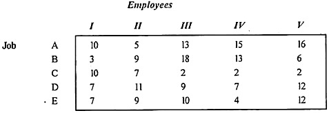
How do I need to assign one job to each employee to minimize total man-hours?

A12)

Applying step (1) and step (2) of the algorithm (2) gives an opportunity reduction time matrix as shown in Table (1).

In the reduced table (1), the minimum time elements in columns I, II, III, IV, and V are 0, 0, 0, 0, 0, respectively, and we subtract these from each element. The columns get the same reduced matrix.

Step 3 (a):

Examine all rows one at a time, starting with A and until you find a row that contains only a single zero element H. All zeros in the assigned column are deleted, as shown in Table 2.

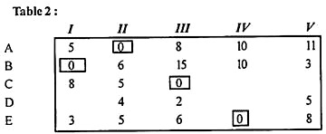
(B) Now, start with the columns and examine each column. 1. There is one zero in column III. Cell (C, III) Allocation is made in this cell. Therefore, cells (C, V) are crossed off. As shown in Table 2, all zeros in the table are assigned or cleared.

The solution is not optimal as only four assignments are made.

Step 4:

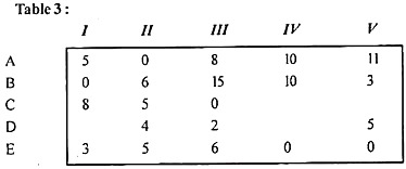
Cover zeros with the minimum number of rows (= 4), as described below.

(A) Line D has no assignment, so mark line (√) line D.

(B) Mark (√) columns I and IV because row D has zero elements in these columns.

(C) Mark (√) rows B and E because (c) columns 1 and (IV) have assignments for rows B and E, respectively.

(D) Draw a straight line through unmarked rows A and C and marked columns I and IV, as other rows or columns cannot be marked, as shown in Table 3.

Step 5:

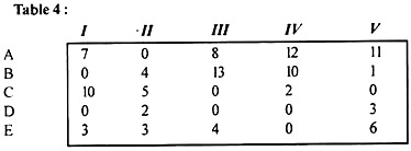
Create a new revised table by selecting the smallest element from all the uncovered elements in the rows of Table 3. , 1), (A, IV), (C, 1) <and (E, IV) respectively. It is at the intersection of the two lines. Table 4 shows another revised table thus obtained.

Step 7:

Repeat steps (3) through (5) to find a new solution. The new assignments are shown in Table 5.

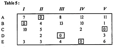
The solution is best if the number of allocations (= 5) is equal to the number of rows (or columns).

The patterns of allocation between jobs and employees and their respective hours (in hours) are shown below.

Q13) Below is a timetable for airlines that operate seven days a week. Crew members must have a flight interval of at least 6 hours. Get a pair of flights that minimizes transit time from home. With any pairing, the crew is based in one city, resulting in fewer connections.

A13)

If your crew is based in Delhi, first create a table of possible connections between flights. The time difference between Flight I and Flight 101 is 24 hours. That is 1,440 minutes, but the minimum transfer required is 6 hours or 360 minutes.

If the crew is based in Delhi, the layover table would look like this:

Similarly, create a transit table for Calcutta-based crew members.

According to the given constraints, the minimum layover times are shown in the following table.

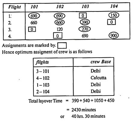
The circled numbers indicate the connections of the Calcutta-based crew, while the encircled numbers indicate the Delhi-based crew.

Step 1:

Subtracting the minimum element of each row from all the elements of the corresponding row gives:

Step 2:

Subtract the column that is minimum from all elements of the column.

Step 3:

Since optimal allocation is not possible in a given situation, assigning to a zero element draws a minimum number of horizontal or vertical lines to cover all zeros, and three as shown below. Get the line.

This number is not equal to the number of rows / columns, so 3 rows are retrieved. The solution is not optimal. Proceed to step (4).

Step 4:

Identify the smallest uncovered element and subtract it from all uncovered elements. In addition to the intersection elements, the matrix is ​​modified as follows (minimum element = 60).

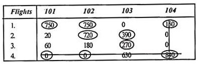
Step 5:

(Repeat step 3) Draw a horizontal vertical line to cover all zeros:

The number of rows is now equal to the row sequence (that is, 4). Therefore, the solution is optimal. Proceed to step (6).

Step 6:

Assign to zero element

Q14) Five salesmen are to be assigned to five districts. Estimates of sales revenue (in thousands) for each salesman are given as follows-

Find the assignment pattern that maximises the sales revenue.

A14)

In order to maximize the sales revenue we have to convert this into minimisation form before proceeding to the Hungarian method.

For this, we obtain the opportunity loss matrix by subtracting every element in the given table from the largest element in it. In this case, the largest element is 41.

Thus, we obtain the following opportunity loss matrix:

Now we apply Hungarian method, we get-

Since the number of assigned zeroes is less than the number of rows, we apply next step of the Hungarian method and draw the minimum number of horizontal/vertical lines that cover all the zeroes as shown in the following

Table-

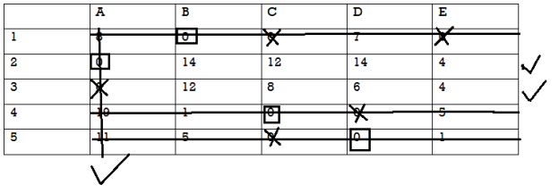
Select the minimum element from amongst the uncovered elements, which is 4 in this case. We subtract the element 4 from each of the uncovered elements and add it to the elements which lie at the intersection of the horizontal and vertical lines. Other covered elements remain unaltered.

Then applying the Hungarian method to the resulting matrix, we get

Since the number of assigned zeroes is equal to the number of rows, the optimum assignment has been attained and is given as:

1 B, 2A, 3E, 4C, 5D

So that, the maximum sales revenue = 38 + 40 + 37 + 41 + 35 thousand rupees

= 191 thousand rupees.