UNIT 1
Demand and Consumer Behaviour
Q1) Explain concept of revenue.
A1)
The term revenue refers to income obtained by the firm through sale of goods and services at different prices
Definition
In the words of Dooley, ‘the revenue of a firm is its sales, receipts or income’.
Revenue are of 3 types as given below

- Total Revenue
- Income received by the seller after selling the output is called total revenue
- “Total revenue is the sum of all sales, receipts or income of a firm.” Dooley
- TR = Q x P
Where,
TR – Total Revenue
Q – Quantity of sale (units sold)
P – Price per unit of output
2. Average Revenue
- Refers to revenue earned by the seller be selling the per unit of commodity
- “The average revenue curve shows that the price of the firm’s product is the same at each level of output.” Stonier and Hague
- AR=TR/Q
Where, AR – Average Revenue, TR – Total Revenue – Total units sold
3. Marginal revenue
- Marginal revenue is the net revenue the firm receives by selling an additional unit of the commodity.
- “Marginal revenue is the change in total revenue which results from the sale of one more or one less unit of output.” Ferguson.
- MR=Change in TR/ change in unit sold
Q2) Explain Revenue under conditions of Perfect and imperfect competition.
A2)
The term revenue refers to income obtained by the firm through sale of goods and services at different prices
Definition
In the words of Dooley, ‘the revenue of a firm is its sales, receipts or income’.
Revenue are of 3 types as given below

- Total Revenue
- Income received by the seller after selling the output is called total revenue
- “Total revenue is the sum of all sales, receipts or income of a firm.” Dooley
- TR = Q x P
Where,
TR – Total Revenue
Q – Quantity of sale (units sold)
P – Price per unit of output
2. Average Revenue
- Refers to revenue earned by the seller be selling the per unit of commodity
- “The average revenue curve shows that the price of the firm’s product is the same at each level of output.” Stonier and Hague
- AR=TR/Q
Where, AR – Average Revenue, TR – Total Revenue – Total units sold
3. Marginal revenue
- Marginal revenue is the net revenue the firm receives by selling an additional unit of the commodity.
- “Marginal revenue is the change in total revenue which results from the sale of one more or one less unit of output.” Ferguson.
- MR=Change in TR/ change in unit sold
Revenue Curve under Perfect competition:
Perfect competition is the term applied to a situation in which the individual buyer or seller (firm) represent such a small share of the total business transacted in the market that he exerts no perceptible influence on the price of the commodity in which he deals.
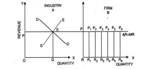
Thus, in perfect competition an individual firm is price taker, because the price is determined by the collective forces of market demand and supply which are not influenced by the individual. When price is the same for all units of a commodity, naturally AR (Price) will be equal to MR i.e., AR = MR. The revenue schedule for a competitive firm is shown in the table

In table we find that as output increases, AR remains the same i.e. Rs. 5. Total revenue increases but at a constant rate. Marginal revenue is also constant i.e. Rs. 5 and is equal to AR.
Thus
TR = AR x Q
Also TR = MR x Q [Since AR = MR]
In figure below, on the X-axis, we take quantity whereas on Y-axis, we take revenue. At price OP, the seller can sell any amount of the commodity. In this case the average revenue curve is the horizontal line. The Marginal Revenue curve coincides with the Average Revenue.
It is because additional units are sold at the same price as before. In that case AR = MR. A noteworthy point is that OP price is determined by demand and supply of industry.
Revenue Curves under Monopoly:
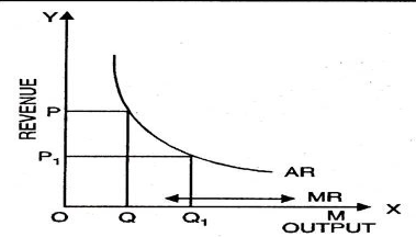
Monopoly is opposite to perfect competition. Under monopoly both AR and MR curves slope downward. It indicates that to sell more units of a commodity, the monopolist will have to lower the price. This can be shown with the help of table.

Revenue Schedule for a Firm under MonopolyIn case of pure monopoly, AR curve can be rectangular hyperbola as has been shown in Fig. In this situation, a producer is so powerful that by selling his output at different prices, he can make the consumer spend his income on the concerned commodity. In this case AR curve is rectangular hyperbola. It implies that TR of the monopolist will remain same whatever may be the price. Area below each point of AR curve will be equal to each other. When TR is constant MR curve will be represented by OX-axis as has been shown in figure.
Q3) Explain elasticity of demand?
A3)
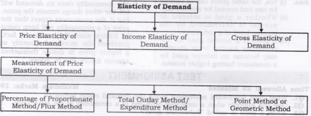
Elasticity of demand
Under law of demand, price falls and demand rises, vice versa. But how much the quantity rise or fall for a given change in price is not determined in law of demand. So the concept of elasticity of demand is derived to know how much quantity demanded changes for a change in the price of goods or services.
“The elasticity (or responsiveness) of demand in a market is great or small according as the amount demanded increases much or little for a given fall in price, and diminishes much or little for a given rise in price”. – Dr. Marshall.
Elasticity means sensitivity of demand to the change in price.
The formula for calculating elasticity of demand is:
EP = proportional changes in quantity demanded/proportional changes in price
Price elasticity of demand
The price of elasticity demand is the change in the quantity demanded to the change in the price of the commodity
Dr Marshall has defined price elasticity of demand as below:
"Price elasticity of demand is a ratio of proportionate changes in the quantity demanded of a commodity to a given proportionate change in its price."
Thus, pride elasticity is responsiveness of change in demand due to a change in price only. Other factors such as income, population, tastes, habits, fashions, prices of substitute and complementary goods are assumed to be constant.
Formula –
Ep = percentage change in quantity demanded/percentage change in price
Types
There are 5 types of price elasticity of demand given below
- Perfectly elastic demand
- A small change in price results to major change in demand is said to be perfectly elastic demand
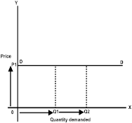
- The demand curve in perfectly elastic demand represent horizontal straight line
- Ep = infinity

From the above figure, we can see at price P1 consumers are ready to buy as much quantity as they want. A slight increase in price may result to fall in demand to zero.
2. Perfectly inelastic demand
- When there is no change in the demand of the commodity with the change in price is said to be perfectly inelastic demand
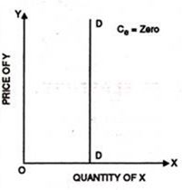
- The demand curve in perfectly elastic demand represent Vertical straight line
- Ep = zero


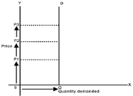
From the above fig, we can see that price is rising from P1 to P2 to P3, but there is no change in the demand. This cannot happen in practical situation. But, in essential goods such as salt, with the change in price the demand does not change.
3. Relatively elastic demand
- When the proportionate change in demand is greater than the proportionate change in price of a product
- The value ranges between one to infinity (ep>1)
- Ex – a smaller change in flight price result in more demand for booking the flight tickets
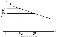

- From the above figure, it is observed that the percentage change in demand from Q2 to Q1 is larger than the percentage change in price from P2 to P1. Thus the demand curve is gradually sloping downwards
4. Relatively inelastic demand
- When the percentage change in demand is less than the percentage change in price
- The value ranges between zero to one (ep<1)
- Ex – cloths, drinks, food, oil , as the change in price does not affect the quantity demanded.

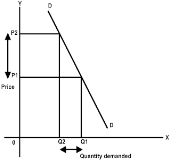
- From the above figure, it is interpreted that the proportionate change in demand from Q2 to Q1 is less than the proportionate change in price from P2 to P1. Thus the demand cure rapidly sloping down.
5. Unitary elastic demand
- When the percentage change in quantity demanded in equal to the percentage change in price of the commodity
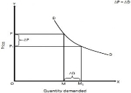
- The value is equal to one (ep=1)

In the above figure we can observe that proportionate change in price from P to P1 cause the same proportionate change in price from M to M1
Income elasticity of demand
The income elasticity is measures the sensitivity of quantity demanded for a goods or services to a change in consumer’s income
 Formula - Percentage change in the quantity demanded
Percentage change in the consumer’s income
Types
- Positive income elasticity of demand -
When a proportionate change in the income of a consumer increases the demand for a product and vice versa, income elasticity of demand is said to be positive. In case of normal goods, the income elasticity of demand is generally found positive.

In Figure, DYDY is the curve representing positive income elasticity of demand. The curve is sloping upwards from left to the right, which shows an increase in demand (OQ to OQ1) as a result of rise in income (OB to OA).
2. Negative income elasticity of demand –
When a proportionate change in the income of a consumer results in a fall in the demand for a product and vice versa, income elasticity of demand is said to be negative. In case of inferior goods, the income elasticity of demand is generally found negative.
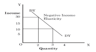
In Figure, DYDY is the curve representing negative income elasticity of demand. The curve is sloping downwards from left to the right, which shows a decrease in the demand as a result of a rise in income. As shown in Figure, with a rise in income from 10 to 30, the demand falls from 3 to 2.
3. Zero income elasticity of demand –
When a proportionate change in the income of a consumer does not bring any change in the demand for a product, income elasticity of demand is said to be zero. It generally occurs for utility goods such as salt, kerosene, electricity.

In Figure, DYDY is the curve representing zero income elasticity of demand. The curve is parallel to Y-axis that shows no change in the demand as a result of a rise in income. As shown in Figure, with a rise of income from 10 to 20, the demand remains the same i.e. 4.
Cross elasticity of demand
“The cross elasticity of demand is the proportional change in the quantity of X good demanded resulting from a given relative change in the price of a related good Y” Ferguson
It measures the percentage change in the quantity demanded of commodity X to the percentage change in the price of its substitute/complement Y
 Formula – proportionate change in quantity demanded of X
Proportionate change in the price of Y
Types
- Positive - When goods are substitute of each other then cross elasticity of demand is positive. In other words, when an increase in the price of Y leads to an increase in the demand of X. For instance, with the increase in price of tea, demand of coffee will increase.
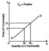
In the above figure, at price OP of Y-commodity, demand of X-commodity is OM. Now as price of Y commodity increases to OP1 demand of X-commodity increases to OM1 Thus, cross elasticity of demand is positive.
2. Negative - A proportionate increase in price of one commodity leads to a proportionate fall in the demand of another commodity because both are demanded jointly refers to negative cross elasticity of demand.

When the price of commodity increases from OP to OP1 quantity demanded falls from OM to OM1. Thus, cross elasticity of demand is negative.
3. Zero - Cross elasticity of demand is zero when two goods are not related to each other. For instance, increase in price of car does not effect the demand of cloth. Thus, cross elasticity of demand is zero.
Q4) Explain price elasticity of demand?
A4)
Price elasticity of demand
The price of elasticity demand is the change in the quantity demanded to the change in the price of the commodity
Dr Marshall has defined price elasticity of demand as below:
"Price elasticity of demand is a ratio of proportionate changes in the quantity demanded of a commodity to a given proportionate change in its price."
Thus, pride elasticity is responsiveness of change in demand due to a change in price only. Other factors such as income, population, tastes, habits, fashions, prices of substitute and complementary goods are assumed to be constant.
Formula –
Ep = percentage change in quantity demanded/percentage change in price
Types
There are 5 types of price elasticity of demand given below
- Perfectly elastic demand
- A small change in price results to major change in demand is said to be perfectly elastic demand
- The demand curve in perfectly elastic demand represent horizontal straight line
- Ep = infinity
From the above figure, we can see at price P1 consumers are ready to buy as much quantity as they want. A slight increase in price may result to fall in demand to zero.
2. Perfectly inelastic demand
- When there is no change in the demand of the commodity with the change in price is said to be perfectly inelastic demand
- The demand curve in perfectly elastic demand represent Vertical straight line
- Ep = zero


From the above fig, we can see that price is rising from P1 to P2 to P3, but there is no change in the demand. This cannot happen in practical situation. But, in essential goods such as salt, with the change in price the demand does not change.
3. Relatively elastic demand
- When the proportionate change in demand is greater than the proportionate change in price of a product
- The value ranges between one to infinity (ep>1)
- Ex – a smaller change in flight price result in more demand for booking the flight tickets


- From the above figure, it is observed that the percentage change in demand from Q2 to Q1 is larger than the percentage change in price from P2 to P1. Thus the demand curve is gradually sloping downwards
4. Relatively inelastic demand
- When the percentage change in demand is less than the percentage change in price
- The value ranges between zero to one (ep<1)
- Ex – cloths, drinks, food, oil , as the change in price does not affect the quantity demanded.


- From the above figure, it is interpreted that the proportionate change in demand from Q2 to Q1 is less than the proportionate change in price from P2 to P1. Thus the demand cure rapidly sloping down.
5. Unitary elastic demand
- When the percentage change in quantity demanded in equal to the percentage change in price of the commodity
- The value is equal to one (ep=1)
In the above figure we can observe that proportionate change in price from P to P1 cause the same proportionate change in price from M to M1
Q5) Explain income elasticity of demand?
A5)
Income elasticity of demand
The income elasticity is measures the sensitivity of quantity demanded for a goods or services to a change in consumer’s income
 Formula - Percentage change in the quantity demanded
Percentage change in the consumer’s income
Types
- Positive income elasticity of demand -
When a proportionate change in the income of a consumer increases the demand for a product and vice versa, income elasticity of demand is said to be positive. In case of normal goods, the income elasticity of demand is generally found positive.

In Figure, DYDY is the curve representing positive income elasticity of demand. The curve is sloping upwards from left to the right, which shows an increase in demand (OQ to OQ1) as a result of rise in income (OB to OA).
2. Negative income elasticity of demand –
When a proportionate change in the income of a consumer results in a fall in the demand for a product and vice versa, income elasticity of demand is said to be negative. In case of inferior goods, the income elasticity of demand is generally found negative.

In Figure, DYDY is the curve representing negative income elasticity of demand. The curve is sloping downwards from left to the right, which shows a decrease in the demand as a result of a rise in income. As shown in Figure, with a rise in income from 10 to 30, the demand falls from 3 to 2.
3. Zero income elasticity of demand –
When a proportionate change in the income of a consumer does not bring any change in the demand for a product, income elasticity of demand is said to be zero. It generally occurs for utility goods such as salt, kerosene, electricity.

In Figure, DYDY is the curve representing zero income elasticity of demand. The curve is parallel to Y-axis that shows no change in the demand as a result of a rise in income. As shown in Figure, with a rise of income from 10 to 20, the demand remains the same i.e. 4.
Q6) Explain cross elasticity of demand?
A6)
Cross elasticity of demand
“The cross elasticity of demand is the proportional change in the quantity of X good demanded resulting from a given relative change in the price of a related good Y” Ferguson
It measures the percentage change in the quantity demanded of commodity X to the percentage change in the price of its substitute/complement Y
 Formula – proportionate change in quantity demanded of X
Proportionate change in the price of Y
Types
4. Positive - When goods are substitute of each other then cross elasticity of demand is positive. In other words, when an increase in the price of Y leads to an increase in the demand of X. For instance, with the increase in price of tea, demand of coffee will increase.

In the above figure, at price OP of Y-commodity, demand of X-commodity is OM. Now as price of Y commodity increases to OP1 demand of X-commodity increases to OM1 Thus, cross elasticity of demand is positive.
5. Negative - A proportionate increase in price of one commodity leads to a proportionate fall in the demand of another commodity because both are demanded jointly refers to negative cross elasticity of demand.

When the price of commodity increases from OP to OP1 quantity demanded falls from OM to OM1. Thus, cross elasticity of demand is negative.
6. Zero - Cross elasticity of demand is zero when two goods are not related to each other. For instance, increase in price of car does not effect the demand of cloth. Thus, cross elasticity of demand is zero.

Q7) Explain indifference curve analysis?
A7)
Indifference curve analysis
Utility analysis suffers from a flaw in the subjective nature of utility, that is, the inability to measure utility quantitatively and accurately. To overcome this difficulty, economists developed a different approach based on the indifference curve. According to this indifference curve analysis, utility cannot be accurately measured, but the consumer can state which of the combinations of two goods he prefers, without describing the magnitude of the strength of his preference. This means that if the consumer is presented with a number of different combinations of goods, he can order or rank them on a “scale of preference “if the different combinations are marked a, B, C, D, E, etc. In this case, the consumer can tell whether he likes A to B or B to A or is indifferent between them. Similarly, he can show his preference or indifference between other pairs or combinations. The concept of order utility means that consumers cannot go beyond stating their preferences or indifference. In other words, if consumers prefer A to B, they don't know by “how much “they prefer A to B. Consumers cannot state the “quantitative difference “between different satisfaction levels. He can simply compare them “qualitatively". That is, it is possible to determine whether simply one satisfaction is higher than another, or lower, or equal.
The basic tool of the Hicks-Allen order analysis of demand is the indifference curve, which represents all those combinations of goods that give the consumer the same satisfaction. In other words, all the combinations of goods that lie on the consumer's indifference curve are equally preferred by him. The independence curve is also known as the Iso-utility curve. Indifferent schedules are tabular statements showing different combinations of two goods that bring the same level of satisfaction.
Table Indifference schedule
Combination Rice (X) Wheat (Y)

I | 1 | 12 |
II | 2 | 8 |
III | 3 | 5 |
IV | 4 | 3 |
V | 5 | 2 |
Now consumers are asked to tell the amount of wheat (Y) they are willing to give up the benefit of an additional unit of rice (X) so that the level of satisfaction remains the same. If the profit of one unit of rice fully compensates for the loss of 4 units of wheat, then the following combination of 2 units of rice
And eight units of wheat will give him as much
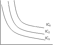
Satisfaction as the first or first combination. A set of indifferent curves representing the size of preference at different levels of satisfaction are understood because the indifferent curve map (below figure).
Although the combination lying on the indifferent curve 3 (IC3) provides the same satisfaction
Product X
Commodity X
Indifference Curve Map
In the above Figure indifference curve map
The level of satisfaction in the indifference curve 3 (IC3) is greater than the level of Satisfaction with indifference curve 2(IC2).
I) the nature of the indifference curve
A) Downward inclination: the indifference curve tilts downwards from left to right.
This means that when the amount of one good in a combination increases, the amount of another must necessarily be reduced so that the total satisfaction is constant.
If the indifference curve is a horizontal straight line (parallel to the X-axis),
Then the indifference curve is a horizontal straight line (parallel to the X-axis),
As shown in the below figure (a) means that as the amount of good X increases,
The amount of good Y will remain constant, but the consumer will remain
Indifferent among the various combinations.
This cannot be done, because consumers always prefer
A large amount of good to a small amount of its good.
Similarly, the indifference curve cannot be a vertical straight line


 Commodity X Commodity X Commodity X
(a) Horizontal Fig.2.4 (b) Vertical Fig.2.4(c) Upward Sloping
Indifference Curve Indifference Curve Indifference Curve
A vertical straight line means that while the amount of good y in combination increases the amount of good X remains constant. The third possibility for the curve is to lean upward to the right.
B) Higher indifference curve gives greater level of utility:
As long as marginal utility of a commodity is positive, an individual will always prefer more of that commodity, as more of the commodity will increase the level of satisfaction.
Combination | Quantity of bananas | Quantity mangoes |
A | 1 | 10 |
B | 2 | 10 |
C | 3 | 10 |
Consider the different combination of bananas and mangoes, A, B and C depicted in table 2.4 and figure 2.7. Combinations A, B and C consist of same quantity of mangoes but different quantities of bananas. Since combination B has more bananas than A, B will provide the individual a higher level of satisfaction than A. Therefore, B will lie on a higher indifference curve than A, depicting higher satisfaction.
Likewise, C has more bananas than B (quantity of mangoes is the same in both B and C). Therefore, C will provide higher level of satisfaction than B, and also lie on a higher indifference curve than B.
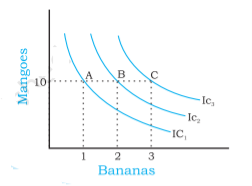
A higher indifference curve consisting of combinations with more of mangoes, or more of bananas, or more of both, will represent combinations that give higher level of satisfaction.
- Two indifference curves never intersect with each other
Two indifference curves intersecting each other will lead to conflicting results. To explain this, let us allow two indifference curves to intersect each other as shown in the figure 2.8. As points A and B lie on the same indifference curve IC1, utilities derived from combination A and combination B will give the same level of satisfaction. Similarly, as points A and C lie on the same indifference curve IC2, utility derived from combination A and from combination C will give the same level of satisfaction.
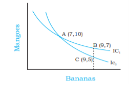
From this, it follows that utility from point B and from point C will also be the same. But this is clearly an absurd result, as on point B, the consumer gets a greater number of mangoes with the same quantity of bananas. So consumer is better off at point B than at point C. Thus, it is clear that intersecting indifference curves will lead to conflicting results. Thus, two indifference curves cannot intersect each other.
Q8) Explain consumer equilibrium?
A8)
Consumer equilibrium
Indifferent map-shows the scale of consumer preferences between various combinations of two goods
Budget line-he shows his money income and various combinations that can afford to buy at the price of both goods.
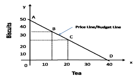
Suppose that the consumer has Rs.20 to spend on tea and biscuits, which cost 50 paise and 40 paise respectively. The consumer has three alternative possibilities before him.
- He may decide to buy tea only, in which case he can buy 40 cups of tea.
- He may decide to buy biscuits only, in which case he can buy 50 biscuits.
- He may decide to buy some quantity of both the goods, say 20 cups of tea (Rs.10) and 25 biscuits (Rs.10) or 12 cups of tea (Rs.6) and 35 biscuits (Rs.14), and so on. (Total amount = Rs.20).
The below figure shows the indifference map with 5 indiscriminate curves (ic1, IC2, IC3, IC4, and IC5) and the budget lines PL for good X and good Y. In order to maximize his level of satisfaction, the consumer tries to reach the highest indifference curve. We assume budget constraints, so he will be forced to stay on the budget line.
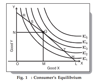
So, what kind of combination is it?
Let's say he chose the combination R from the figure. 1, we see that R is on the low indifference curve–IC1. He can easily afford the combination S, Q, or T that is on a high Ic. Even if he chooses the combination H, the argument is similar because H is on the curve IC1.
Next, let's check out the mixture S lying on the curve IC2. Again, he can reach a better level of satisfaction within the budget by choosing the mixture Q lying on IC3–the argument is analogous for the mixture T, since the higher T is also on the curve IC2.
Therefore, we have left the combination Q.
What happens when he chooses the combination Q?
This is the simplest choice because Q is on his budget line and pts puts him on the simplest possible indifference curve, IC3. There are higher curves, IC4 and IC5, but they are over his budget. Thus, he reaches equilibrium at the point Q on the curve IC3.
Note that at this point the budget line PL is bordered by the indifference curve IC3. Also in this position, consumers buy X in OM amount and Y in ON amount.
Since Point Q is tangent, the slope of line PL and curve IC3 is equal at this point. In addition, the slope of the indifference curve shows that the substitution limit rate (MRSxy) of X with respect to Y is
Hence, at the equilibrium point Q,
MRSxy = MUxMUyMUxMUy = PxPy
Also, the slope of the price line (PL) shows the ratio of X and Y prices. Therefore, we can say that the consumer equilibrium is achieved when the price line is bordered by the indifference curve. Alternatively, when the substitution limit rate of goods X and Y is equal to the ratio between the prices of two goods.
Q9) Explain price consumption curve?
A9)
Price consumption curve
The price consumption curve(PCC) shows the varying amounts of products purchased by consumers as their prices change. The marshalian demand curve also shows different amounts of products demanded by consumers at various prices, while others remain an equivalent .
Given the income of the consumer's money and his indifference map, it's possible to draw a requirement curve for any commodity from the PCC.The conventional demand curve is straightforward to draw from a given price demand schedule for a commodity, whereas the drawing of the demand curve from the PCC is somewhat complicated. However, the latter method has more edges than the previous . It reaches an equivalent result without making dubious assumptions of the measurable utility of utility and therefore the constant utility of cash .
The derivation of the demand curve from the PCC also explains the income and alternative effects of a given decline or rise within the price of products that the Marshallian demand curve can't be explained. Therefore, the ordinal method for deriving the demand curve is superior to the marshalian method.
Assumption:
In this analysis、:
(a) the cash spent by the buyer is given and constant; it's Rs10.
b) the worth of an honest X falls.
(c) the costs of other related products won't change.
(d) consumer preferences and preferences are constant.
In double story figure 38, money is taken in rupees on the vertical axis and an honest X on the horizontal axis. PQ,PQ1 and PQ2 are the budget lines of consumers where R, S and T are the equilibrium positions forming the PCC curve, and if the entire gold income of consumers in OA, OB and OC units of X respectively at these points on the PCC curve divided by the amount of products purchased with it, we get per unit price of excellent . For X, OA unit, he pays OP/OQ price;for OB unit,OP/OQ1 price; and for OC unit, OP / OQ2.This is, in fact, the buyer price demand schedule for the great X shown in Table 5..
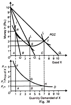
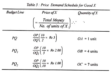
Consumer price demand for an honest X schedule shows that given his money income OP (Rs.10) when he spends his income on buying an oq amount (2 units), it means the worth of X is OP/OQ (Rs).5) consumers buy an honest X OA (one unit) per budget line PQ this is often indicated by the purpose R on the F curve.
If OP/OQ is valued by A, by the budget line PQ (Rs. 2), the worth consumption curve shows that he buys X OB (4 units). When the worth of excellent X is decided as OP/OQ2(=Re1)as the budget line PQ2 and therefore the curve L at the purpose T, the buyer buys OC(7 units)of X.Points R, S,and T on the PCC curve indicate the price-quantity relationship permanently X.
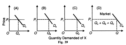
These points are plotted in the figure below figure 38. The price of X is the amount taken on the vertical axis and required on the horizontal axis. To draw a demand curve from PCC, draw a vertical from the top point R in Figure 38 to the bottom figure that should pass through point A, and then draw a line at point P1 (=5) on the price axis (figure below).
Points G and H are drawn in a similar way. This curve shows the amount of X that consumers demand at different prices. As the price of X falls, consumers buy more units of it, and the demand curve D tilts downward to the right.
Q10) Explain income consumption and Engel curve?
A10)
Income consumption curve and Engel curve
With given money income and prices of two commodities the consumer will be in equilibrium at the tangency point between the budget line and the highest indifference curve. Now, we will analyze how the situation changes and the consumer attains a new equilibrium, when income changes without any change in goods’ prices. The income consumption curve is the locus of all consumer equilibrium points resulting due to changes in consumer’s income only, with prices remaining unchanged.
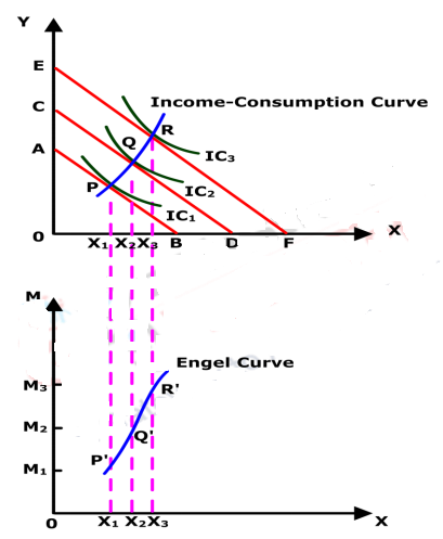
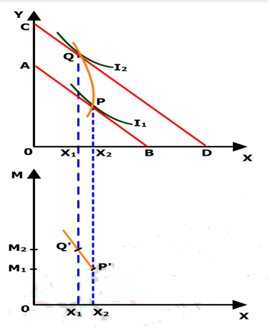
In the below figure , AB indicates the budget line for a given income level (M1) and given prices. The consumer is in the equilibrium at point P when indifference curve IC1 is tangent to the budget line AB. At P, the consumer purchases OX1 of commodity X and OY1 of commodity Y. Now, suppose the income of the consumer increases from M1 to M2. With this increase in income the consumer would now be able to purchase larger quantities of both the commodities. As a result, the budget line shifts rightward, parallel to the original budget line AB. The new budget line representing M2 income level is shown by CD. With the budget line CD the consumer reaches a new equilibrium Q on the highest possible indifference curve IC2. At Q the consumer purchases OX2 of commodity X and OY2 of commodity Y. Thus, as a result of increase in income the consumer purchases more of both the commodities. At the higher indifference curve IC2 the consumer satisfaction increases, so that he is better off at Q as compared to P. If his income increases further to M3 so that the budget line shifts to EF, the consumer reaches the indifference curve IC3 at point R and purchases greater quantities of both the commodities. If the successive consumer equilibrium points (like P, Q and R) corresponding to various level of income are connected together, we obtain the Income Consumption Curve (ICC). The Income Consumption Curve is thus the locus of the consumer’s equilibrium points corresponding to different levels of consumer’s income.

Engel curve
The income consumption curve can be used to derive the relationship between a consumer’s income and the quantity of goods purchased. The Engel curve shows the relationship between the consumer’s level of income and quantity purchased of a commodity, other factors remaining constant.
To derive the Engel curve from income consumption curve let us measure income levels on the vertical axis and quantity of a good purchased on the horizontal axis as in the lower panel of above Figure. The Income Consumption Curve in the top panel of above figure shows the equilibrium quantity of X and Y purchased as the income level changes. The parallel budget lines AB, CD and EF corresponds to M1, M2 and M3 level of income respectively, prices remaining constant. Each point of the ICC corresponds to a particular level of income and to a particular quantity of X (and Y). The various combinations of the income level and the quantity purchased of good X i.e. (M1, OX1), (M2, OX2) and (M3, OX3) are plotted in the lower panel to obtain the Engel curve for good X. The income-quantity combinations (M1, OX1), (M2, OX2) and (M3, OX3) shown by point P’, Q’ and R’ in the lower panel of Figure 1 correspond to the consumer’s equilibrium points P, Q and R respectively in the top panel of above figure.
In case of a normal good the consumer purchases more of it when his income increases. But an inferior good is a type of good which the consumer purchases less of when his income increases.
Above fig shows the income consumption curve and Engel curve when X is a normal good. We get a positively sloped Engel curve and income consumption curve for a normal good because the consumer purchases more of X when his income increases.
Now, let us assume X is an inferior good given in below figure. In this case, consumption of the commodity decreases as income increases. So the ICC is backward bending and the Engel curve is negatively sloped, indicating a fall in quantity purchased with an increase in income.
The income consumption curve is obtained by joining the different consumer equilibrium points as income increases from M1 to M2. As money income increases the consumer equilibrium moves from the point P on I 1to point Q on a higher indifference curve I2. At the new equilibrium Q the consumer purchases less of commodity X, which is an inferior good and more of commodity Y which is a normal good. This generates a negatively sloped income consumption curve PQ. The corresponding Engel curve is derived in the lower panel of below figure. We obtain a negatively sloped Engel curve since an increase in income leads to a decline in quantity purchased of the inferior good X.

Q11) Explain engel curve?
A11)
Engel curve
The income consumption curve can be used to derive the relationship between a consumer’s income and the quantity of goods purchased. The Engel curve shows the relationship between the consumer’s level of income and quantity purchased of a commodity, other factors remaining constant.
To derive the Engel curve from income consumption curve let us measure income levels on the vertical axis and quantity of a good purchased on the horizontal axis as in the lower panel of above Figure. The Income Consumption Curve in the top panel of above figure shows the equilibrium quantity of X and Y purchased as the income level changes. The parallel budget lines AB, CD and EF corresponds to M1, M2 and M3 level of income respectively, prices remaining constant. Each point of the ICC corresponds to a particular level of income and to a particular quantity of X (and Y). The various combinations of the income level and the quantity purchased of good X i.e. (M1, OX1), (M2, OX2) and (M3, OX3) are plotted in the lower panel to obtain the Engel curve for good X. The income-quantity combinations (M1, OX1), (M2, OX2) and (M3, OX3) shown by point P’, Q’ and R’ in the lower panel of Figure 1 correspond to the consumer’s equilibrium points P, Q and R respectively in the top panel of above figure.
In case of a normal good the consumer purchases more of it when his income increases. But an inferior good is a type of good which the consumer purchases less of when his income increases.
Above fig shows the income consumption curve and Engel curve when X is a normal good. We get a positively sloped Engel curve and income consumption curve for a normal good because the consumer purchases more of X when his income increases.
Now, let us assume X is an inferior good given in below figure. In this case, consumption of the commodity decreases as income increases. So the ICC is backward bending and the Engel curve is negatively sloped, indicating a fall in quantity purchased with an increase in income.
The income consumption curve is obtained by joining the different consumer equilibrium points as income increases from M1 to M2. As money income increases the consumer equilibrium moves from the point P on I 1to point Q on a higher indifference curve I2. At the new equilibrium Q the consumer purchases less of commodity X, which is an inferior good and more of commodity Y which is a normal good. This generates a negatively sloped income consumption curve PQ. The corresponding Engel curve is derived in the lower panel of below figure. We obtain a negatively sloped Engel curve since an increase in income leads to a decline in quantity purchased of the inferior good X.
Q12) explain income and substitution effects?
A12)
Income and substitution effect
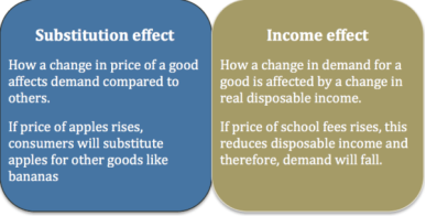
A good increase in prices will then have two different effects–known as profit and alternative effects.
If a good increase in price
- Goods are relatively more expensive than alternatives, and therefore people will switch to other goods that are relatively inexpensive. (Substitution effect)
- Higher prices reduce disposable income, and this low income can reduce demand. (Income effect)
Substitution effect
It states that the increase in the price of good will encourage consumers to buy alternative goods. The alternative effect measures the amount at which higher prices encourage consumers to buy different goods, assuming the same level of income.
Income effect
Thus price changes affect the interests of consumers. If prices rise, it will effectively cut disposable income and lower demand for good for disposable income this fall.
For example:
When the price of meat rises, the higher the price, consumers can switch to alternative food sources, such as buying vegetables.
But the higher the price of meat, it means that after buying some meat, they have a lower reserve income. Therefore, consumers buy less meat, but this profit.
If it goes well, it will increase like a diamond an alternative diamond for no substitution effect however, the higher the price of a diamond, the lower the demand due to the income effect.
Income and alternative effects on wages
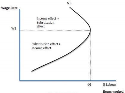
For workers, there is a choice between work and leisure.
When wages rise, work becomes relatively more profitable than leisure time. (Substitution effect)
But with higher wages, he can maintain a decent standard of living through fewer jobs. (Income effect)
The alternative effect of higher pay means workers give up their leisure time to do more hours of work because jobs now have higher rewards.
The income effect of higher wages means that workers spend less time working because they can maintain their target income level in less time.
If the alternative effect is greater than the income effect, people do more work (W1, up to Q1). But we may be at a certain hourly rate where we can afford to work less time. In the figure above, after w1, the income effect is dominant.
It depends on the workers in question. You can enjoy leisure and high-paying jobs. The income effect will soon dominate. If you have a lot of debt and spending commitments, the income effect will take a long time to occur.
Income and alternative effects for interest rates and savings
Higher interest rates increase income from savings. Thus, this will give consumers more income, which can lead to higher spending (income effect)
Higher interest rates make savings more attractive than consumption and reduce consumer spending (alternative effects)
Q13) explain measurement of elasticity of demand
A13)
Elasticity of demand
Under law of demand, price falls and demand rises, vice versa. But how much the quantity rise or fall for a given change in price is not determined in law of demand. So the concept of elasticity of demand is derived to know how much quantity demanded changes for a change in the price of goods or services.
“The elasticity (or responsiveness) of demand in a market is great or small according as the amount demanded increases much or little for a given fall in price, and diminishes much or little for a given rise in price”. – Dr. Marshall.
Elasticity means sensitivity of demand to the change in price.
The formula for calculating elasticity of demand is:
EP = proportional changes in quantity demanded/proportional changes in price

Price elasticity of demand
The price of elasticity demand is the change in the quantity demanded to the change in the price of the commodity
Dr Marshall has defined price elasticity of demand as below:
"Price elasticity of demand is a ratio of proportionate changes in the quantity demanded of a commodity to a given proportionate change in its price."
Thus, pride elasticity is responsiveness of change in demand due to a change in price only. Other factors such as income, population, tastes, habits, fashions, prices of substitute and complementary goods are assumed to be constant.
Formula –
Ep = percentage change in quantity demanded/percentage change in price
Types
There are 5 types of price elasticity of demand given below
- Perfectly elastic demand
- A small change in price results to major change in demand is said to be perfectly elastic demand
- The demand curve in perfectly elastic demand represent horizontal straight line
- Ep = infinity

From the above figure, we can see at price P1 consumers are ready to buy as much quantity as they want. A slight increase in price may result to fall in demand to zero.
2. Perfectly inelastic demand
- When there is no change in the demand of the commodity with the change in price is said to be perfectly inelastic demand
- The demand curve in perfectly elastic demand represent Vertical straight line
- Ep = zero


From the above fig, we can see that price is rising from P1 to P2 to P3, but there is no change in the demand. This cannot happen in practical situation. But, in essential goods such as salt, with the change in price the demand does not change.
3. Relatively elastic demand
- When the proportionate change in demand is greater than the proportionate change in price of a product
- The value ranges between one to infinity (ep>1)
- Ex – a smaller change in flight price result in more demand for booking the flight tickets


- From the above figure, it is observed that the percentage change in demand from Q2 to Q1 is larger than the percentage change in price from P2 to P1. Thus the demand curve is gradually sloping downwards
4. Relatively inelastic demand
- When the percentage change in demand is less than the percentage change in price
- The value ranges between zero to one (ep<1)
- Ex – cloths, drinks, food, oil , as the change in price does not affect the quantity demanded.


- From the above figure, it is interpreted that the proportionate change in demand from Q2 to Q1 is less than the proportionate change in price from P2 to P1. Thus the demand cure rapidly sloping down.
5. Unitary elastic demand
- When the percentage change in quantity demanded in equal to the percentage change in price of the commodity
- The value is equal to one (ep=1)

In the above figure we can observe that proportionate change in price from P to P1 cause the same proportionate change in price from M to M1
Measurements
1. Ratio or Proportional Method
This ratio method of measuring elasticity of demand is also known as Arithmetic or Percentage method. This method is developed by Dr. Marshall. In this method percentage change in quantity demanded and divide it by percentage change in the price of the commodity.
Example
Price of X | Demand (Units) |
200 | 1000 |
100 | 1500 |
In the above table we can see the price of commodity X falls from Rs. 200/- to Rs. 100/- and quantity demanded increases from 1000 units to 1500 units. Here percentage change in demand is 50, whereas percentage change in price is also 50. Therefore, 50%, / 50% = 1, which, means Ed is unitary or one.
2. Total expenditure method - In this method, statistics of total expenditure is used to find out elasticity of demand. Total expenditure at the original price and total expenditure at the new price is compared with each other, and we come to know the elasticity of demand.
When price falls or rises, total expenditure does not change or remains constant, demand is unitary elastic.
When price falls, total expenditure increases or price rises and total expenditure decreases, demand is elastic or elasticity of demand is greater than one.
Example
Price (Rs.) | Demand (Units) | Total Outlay (Rs.) | Elasticity of Demand | |
A | 10 8 | 12 15 | 120 120 | Unitary or 1 |
B | 10 8 | 12 20 | 120 160 | Elastic or > 1 |
C | 10 8 | 12 14 | 120 112 | Inelastic or < 2 |
3. Point elasticity method – the price elasticity of demand also be measured at any point on the demand curve. It is noted that demand is unitary at mid point of demand curve that total revenue is maximum at this point. Any point above unitary point shows elasticity is greater than one (means price relation in this point leads to an increase in the total revenue.
Any point below mid point shows elasticity is less than one means price relation in these point lead to reduction in the total revenue.
Q14) Explain factors affecting price elasticity of demand
A14)
Factors affecting price elasticity of demand
The price elasticity of demand depends upon number of factors which affects its elasticity. They are as follows:
- Nature of goods or commodity: The elasticity of demand for a commodity depends upon the nature of the commodity, i.e., whether the commodity is a necessary, comfort or luxury good. The elasticity of demand for a necessary commodity is relatively small. For example, if the price of such a good rise, its buyers generally are not able to reduce its demand as its necessity commodity.
- Availability of Substitute Goods: The price elasticity of demand also depends upon the substitution of goods. If there is a close substitute for a particular commodity in the market, then the demand for such commodity would be relatively more elastic. For example, since tea and coffee are close substitute for each other in the commodity market, a rise in the price of coffee will result in a considerable fall in its demand and a consequent rise in the demand for tea. Therefore, a demand for coffee will be relatively more elastic because of the availability of tea in the market.
- Alternative and Variety of Uses of the Product: as we know that the resources have an alternative use. The demand for such goods has many uses. The more the alternative and variety of uses of a good, the more would be its elasticity of demand. For example, Electricity is used for many purposes such as lighting, heating, cooking, ironing and also use as a source of power in many industries & households. That is why when the price of electricity increases, its demand will decrease and vice versa.
- Role of Habits and custom: if the consumer has a habit of something, he will not reduce his consumption even if the price of such commodity increases the demand for them do not decreases considerably and so their elasticity of demand will be inelastic. Ex; Alcohol, Cigarettes which are injurious for health but people still consume it because of their habit.
- Income Level of the consumer: The elasticity of demand differs due to the change in the income level of the households. Elasticity of demand for a commodity is low for higher income level groups then the people with low incomes. This is because rich people are not influenced much by changes in the price of goods. Poor people are highly affected by the increase or decrease in the price of goods. As a result, demand for the lower income group is highly elastic in demand.
- Postponement of Consumption: if the consumer postponed the consumption of commodity in future the demand is relatively elastic. For example, commodities whose demand is not urgent, have highly elastic demand as their consumption can be postponed if there is an increase in their prices. However, commodities with urgent demand like medicines have inelastic demand because it is an essential commodity whose consumption cannot be post pended.
- Time Period: Price elasticity of demand is related to a period of time. The elasticity of demand varies directly with the time period. In the short run the demand is generally inelastic and in long-run it becomes relatively elastic. This is because consumers find it difficult to change their habits, in the short run, in order to response to the change in the price of the commodity. However, demand is more elastic in long run as their other substitutes available in the market, if the price of the given commodity rises.
Q15) explain income and cross elasticity of demand?
A15)
Income elasticity of demand
The income elasticity is measures the sensitivity of quantity demanded for a goods or services to a change in consumer’s income
 Formula - Percentage change in the quantity demanded
Percentage change in the consumer’s income
Types
- Positive income elasticity of demand -
When a proportionate change in the income of a consumer increases the demand for a product and vice versa, income elasticity of demand is said to be positive. In case of normal goods, the income elasticity of demand is generally found positive.
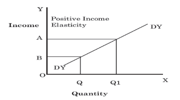
In Figure, DYDY is the curve representing positive income elasticity of demand. The curve is sloping upwards from left to the right, which shows an increase in demand (OQ to OQ1) as a result of rise in income (OB to OA).
2. Negative income elasticity of demand –
When a proportionate change in the income of a consumer results in a fall in the demand for a product and vice versa, income elasticity of demand is said to be negative. In case of inferior goods, the income elasticity of demand is generally found negative.

In Figure, DYDY is the curve representing negative income elasticity of demand. The curve is sloping downwards from left to the right, which shows a decrease in the demand as a result of a rise in income. As shown in Figure, with a rise in income from 10 to 30, the demand falls from 3 to 2.
3. Zero income elasticity of demand –
When a proportionate change in the income of a consumer does not bring any change in the demand for a product, income elasticity of demand is said to be zero. It generally occurs for utility goods such as salt, kerosene, electricity.
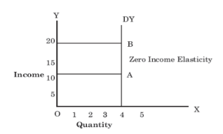
In Figure, DYDY is the curve representing zero income elasticity of demand. The curve is parallel to Y-axis that shows no change in the demand as a result of a rise in income. As shown in Figure, with a rise of income from 10 to 20, the demand remains the same i.e. 4.
Cross elasticity of demand
“The cross elasticity of demand is the proportional change in the quantity of X good demanded resulting from a given relative change in the price of a related good Y” Ferguson
It measures the percentage change in the quantity demanded of commodity X to the percentage change in the price of its substitute/complement Y
 Formula – proportionate change in quantity demanded of X
Proportionate change in the price of Y
Types
- Positive - When goods are substitute of each other then cross elasticity of demand is positive. In other words, when an increase in the price of Y leads to an increase in the demand of X. For instance, with the increase in price of tea, demand of coffee will increase.

In the above figure, at price OP of Y-commodity, demand of X-commodity is OM. Now as price of Y commodity increases to OP1 demand of X-commodity increases to OM1 Thus, cross elasticity of demand is positive.
2. Negative - A proportionate increase in price of one commodity leads to a proportionate fall in the demand of another commodity because both are demanded jointly refers to negative cross elasticity of demand.
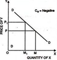
When the price of commodity increases from OP to OP1 quantity demanded falls from OM to OM1. Thus, cross elasticity of demand is negative.
3. Zero - Cross elasticity of demand is zero when two goods are not related to each other. For instance, increase in price of car does not effect the demand of cloth. Thus, cross elasticity of demand is zero.
