Q1) Explain isoquants?

A1)

The term “iso-quants” is derived from Greek word iso means “equal” and quants means “quantity”. Thus, iso-quant means equal quantity. An iso-quant is also known as iso-production curve, iso-indifference, equal production curve by various economists. The isoquants have its properties which are similar to those generally assumed for indifference curve theory of the theory  of consumer’s behaviour analysis. Iso-quant is defined as “a locus of all the combination of two factors of production that yields that yield the same level of output.”

Thus, an iso-quant is a combination of any two factor inputs that represents and produce the same level of output. Any two combinations of input factors e.g. Labour and capital are used in which one factor is increased by decreasing the other factor of input to maintain the same level of production.

Iso-quant can be explained with the schedule and graph given below:

Factor combinations to produce a given level of output

The above table shows the five combination of inputs i.e. Labour and Factor unit which yield the same level of output of 500 units. Which says any point on the iso-quant will give the same level of output. To show this we draw the iso-quant drawn below:

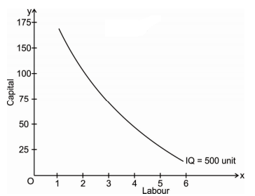
Iso-quant map:

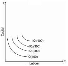
An iso-quant map represents a set of iso-quant curves shows the combination of input factor at the various level of output. A higher level of iso-quant represents the higher level of output. Thus, in simple word, iso-quant map is a family of iso-quant representing the various iso-quant curve at a particular level of output. The iso-quant map can be represented with the diagram given below:

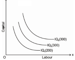
The fig above shows the various iso-quants representing the various level of output at different combination of input factors. IQ1 , IQ2 and IQ3 shows the iso-quant which produces 100,200 and 300 units of output respectively with the various combination of input factors which provides the same level of output at different level of Iso-quant.as we had said higher the Iso-quant represents higher the value of output.

Properties

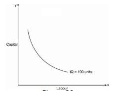
Thus, the iso-quant can be downward sloping from left to right. There can’t be an upward sloping iso-quant curve because it shows that a given product can be produce by using less of both the input factor. Similarly, an iso-quant cannot be horizontal or vertical because it also doesn’t represent the equilibrium position of a firm. Only the downward sloping supply curve represents the characteristics of iso-quant.

2.        Iso-quant are convex to the origin: As we had discussed in the above property that the iso-quant curve is downward sloping and it has a negative slope and it operates under law of Marginal rate of Technical Substitution (MRTS). It says that it equals the ratio of the marginal product if labour and marginal product of capital i.e. one factor is given up to get one additional unit of other factor to produce the same of output which creates a convexity of iso-quant curve.

Thus, the slope of iso-quant can be represented by,

The above equation represents ratio of change in capital and labour should be equal to the ratio of the marginal rate of technical substitution of labour and capital which is equal to the ratio of marginal product of labour and capital.

The convexity of iso-quant means that as we move down the curve less and less of capital given up for an additional unit of labour so to produce the same level of output. The convexity of isoquant can be observed from the diagram Given below

Thus, the iso-quant can be convex to the origin but not the concave because it would mean that MRTS will increase instead of decreasing i.e. labour will increase at a constant rate the amount of capital given up will goes on increasing

3.        Iso-quants do not intersect: The properties of iso-quants say that two iso-quant will never intersect each other. To explain this, we will take a help of following Diagram

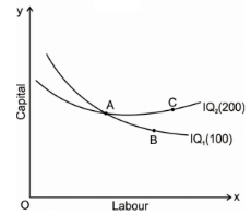
The above fig represents two different iso-quant IQ1and IQ2, where it represents the level of output 100 and 200 units respectively. Point a represents 100 units of output on IQ1 and point c represents 200 units of output on IQ2. The point b shows the intersection of both the iso-quants where is logically not possible to identify the level of output.

4.        Iso-quant cannot touch either of the axis: an iso-quant cannot only touch x axis or y axis or any either axis because it will represent that the iso-quant only produce goods by using one factors of production either by using only capital or only labour which is practically not possible and which is unrealistic.

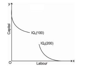
5.        Higher the iso-quant higher the level of production: if there is a multiple iso-quant showing different level of production in one diagram. Where the higher the iso-quant i.e. the iso-quant far from the origin indicates higher level of output and the iso-quant close to the origin indicates lower level of output.

Q2) Explain marginal rate of technical substitution?

A2)

Marginal rate of technical substitution refers to rate, at which one

Input can be substituted for another input, without affecting the total output. Capital and labour are two inputs, in case amount of capital that can be replaced by an extra unit of labour, keeping the output constant.

Marginal rate of technical substitution of labour for capital = slope = ∆K/∆L

.

Capital and labour are not perfect substitutes for each other so The MRTS has decreased. Therefore , while keeping the output level constant, more of labour is added, less  of capital can be used.

Since, by definition, output remains constant on an isoquant the loss in physical output from a small reduction in capital will be equal to the gain in physical output from a small increment in labour.

The loss in output is calculated by multiplying the marginal physical product of capital (MP) by the amount of reduction in capital. The gain in output is calculated by multiplying the marginal physical product of labour (MP by the increment in labour.

Accordingly, along an isoquant:

∆K.MPK + ∆L.MPL = 0

∆K x MPK = ∆L x MPL

∆K/∆L = MPL/MPK

But ∆K/∆L, by definition, is the marginal rate of technical substitution of labour for capital

Therefore, MRTSLK = MPL/MPK

Thus we can see that marginal rate of technical substitution of labour for capital is the ratio of marginal physical product of the two factors labour and capital.

Q3) Explain economic region of production?

A3)

Economic region a territorial component of a country’s national economy. Economic region is characterised by specific economic-geographical status, by an economic unity, by distinctive natural and economic conditions, and by a production specialization based on territorial social division of labor.  Under capitalism, in the heat of competition economic regions form and develop spontaneously. Under socialism, based on the economic laws of socialism, the territorial division of labor develops, and economic regions form develops in a planned fashion.

In the formation of economic regions, specialization within the social territorial division of labor plays the principal role. The boundaries of a region is determined by the specialised branches action and major auxiliary facilities—the associated cooperative suppliers of raw materials, assemblies, and parts.

Economic region is also influenced by natural conditions such as the natural fertility of the soil, and the climate, the presence of large deposits of minerals.

Other factors influencing the economic region formation are administrative and political units , technical and economic conditions.

The three levels of economic regions are as follows: large (macroregions), administrative (mesoregions), and lowest-level (microregions).

Large economic regions comprise three types: Union republics, groups of Union republics, and groups of autonomous republics. The large economy determines territorial proportions of national economies. It also determines the trends in the location of productive forces throughout the national economy.

Administrative economic regions form the basis of the country’s territorial makeup. It includes the basic elements in the territorial planning and management of the national economy.

Lowest-level economic regions are low-level administrative regions that include the primary territorial elements in the classification of economic regions.

Q4) Explain optimal combination of resources?

A4)

Optimum factors of production are explained in two methods are as follows

Formula:

Mppa = Mppb = Mppc = Mppn

  Pa         Pb        Pc        Pn

Where as,

a, b, c, n are different factors of production.

Mpp is the marginal physical product.

A firm compares the Mpp / P ratios with that of another. A firm will reduce its cost by using more of those factors with a high Mpp / P ratios and less of those with a low Mpp / P ratio until they all become equal.

2.        The isoquant approach - The least cost combination of-factors is explained with the help of iso-product curves and isocosts. The optimum factors combination or the least cost combination refers to the combination of factors to produce a specific quantity of output at the lowest possible cost. The least cost combination of factors for any level of output when the iso-product curve is tangent to an isocost curve

The choice of a particular combination of factors depends on technical possibilities of production and the prices of factors used for the production of a particular product.

The prices of factors are represented by the iso-cost line. The Iso cost line is very important in determining what combination of factors the firm will choose for production

For ex,  a firm has to spend 300/-on the factors of production such as labour and capital. Price of labour is Rs. 4 per labour hour and the price of capital is Rs. 5 per machine hour. With outlay of Rs. 300, a firm can buy 75 units of labour or 60 units capital). In the below figure, OB represent 75 units of labour and OA represent 60 units of capital.

This line AB is called iso-cost line, the combination of various factors which a firm can buy with a constant out­lay. The iso-cost line is also called the price line or outlay line.

Assumption of optimum factor combination-

The optimum factor combination is explained in the below diagram

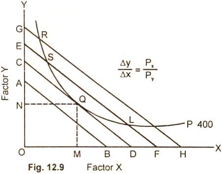
The entrepreneur decides to produce 400units of output which is represented by isoquant P. The 400 unit of output can be produced by any combination of factor X(labour) and Factor Y (capital) such as R, S, Q, L and P lying on the isoquant. For producing 400 units, the cost will be minimum at point Q, which the iso-cost line CD is tangent to the given isoquant. At no other point such as R, S,L, P the cost is minimum. Therefore the firm will not choose any combination of R,S,L,P.

Q5) Explain the expansion path?

A5)

In economics, an expansion path is a line connecting optimal input combinations as the scale of production expands. A producer seeking to produce the most units of a product in the cheapest possible way to increase production along the expansion path.

Definition

Economist Alfred Stonier and Douglas Hague defined expansion path  as,” that line which reflects least cost method of producing different levels of output, when factor prices remains constant”.

Assumption

In order to maximise profits, the firm combines labour and capital in such a way that the ratio of their MP is equal to the ratio of their prices

This occurs at a point of tangency between an isocost line and an isoquant curve.

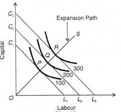
In the above figure, the different isoquant lines areC1L1,C2L2,C3L3. Keeping the prices of factors constant, the different isoquant lines are shown parallel to each other. There are three isoquants ie 100, 200, 300 representing successively higher level of output.

At point P, the firm is at equilibrium, where the isoquant 100 is tangent to its corresponding isoquant line C1L1. Similarly the firm is equilibrium at point Q and R, where the isoquant 200 and 300 is tangent to its corresponding isoquant line C2L2 and C3L3. Each point of tangency implies optimum combination of capital and labour that produces optimum level of output. The line OS joining the equilibrium point P,Q,R from the origin is the expansion path of the firm.

Q6) Explain return of scale using isoquants?

A6)

The laws of returns to scale refer to the long run analysis of production. In the long run all the factors become variable. So output can be expanded by changing all the factors simultaneously, so that the scale of production is changed.

The term  returns to scale refers to the situation of increase in output by increasing all the factors by the same proportion. Firms can choose any scale of production. They can double or triple output or go out of business completely. Return to scale can be constant, increasing or decreasing in the long run.

Constant returns to scale. Technically, the term constant returns, means that the quantitative relationship between input and output stays constant or the same, when output is increased. If a firm doubles its inputs, it doubles output if it triples inputs, it triples output; and so forth.

Furthermore, if input prices are fixed, constant returns implies that the average cost of production does not change with scale: In terms of following diagram I, in constant returns to scale, the isoquants are equidistant along the product line OP, where product line is defined as a line showing movement from one isoquant to another resulting from the change in factor input combinations.

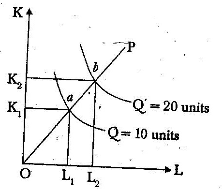
This case, by doubling the capital and labour inputs, the firm is able to double the output at level of 20 units. The distance between consecutive. Multiple isoquants remains the same under constant returns to scale thereforeOa = ab.

Increasing returns to scale. Technically, the phrase increasing returns to scale refers to the relationship between inputs and outputs. When we say that a production function exhibits increasing’returns, we mean that given percentage increase in inputs leads to a larger percentage increase in the production of output.

For example, if a firm doubled or tripled inputs, it would More than double or triple output. When the prices of inputs do not change with output levels, then the increasing.

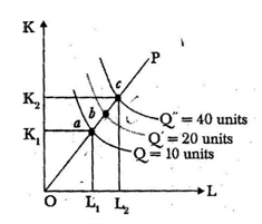
Returns to scale also means that as output rises, average cost of production falls. In terms of the following diagram 2, increasing’returns to scale implies that the distance  between consecutive multiple isoquants decreases along the product line i.e., C a < ab.

Decreasing returns to scale: In this case, increase in output is less than the  increase in inputs in proportionate terms. In terms of diagram, the distance between  successive multiple isoquants increases along the product line OP as shown below :

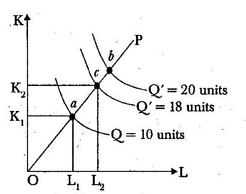
= 20 units Q = 18 units

Q= 10 units.

Li L2 Diagram 3

At the initial combination (L1, K1) at point a on the product line OP, output is 10 units. When the factor inputs are doubled i.e., (L2 K2) at point c, the output is less than doubled i.e., Q’ = 18 units. Whereas doubling the output (Q’ = 20 units) requires more then double of the inputs. So the distance between isoquants has increased, i.e., Oa < ab, indicating decreasing return to stale.

Q7) Explain cost of production?

A7)

Social and private costs of production

Private cost are the those costs that are incurred by the individuals and firms who are directly involved in some economic activity. When goods and services are produced, then certain direct and indirect costs are borne by the producing agents. Examples of private costs are the factors payments made and expenditure on raw materials incurred by the producing agent concerned.

Social cost are the costs incurred by the society as a whole. These are the private costs plus any costs borne by the rest of the society. So social costs are higher than private costs when firms are able to escape some of the economic costs of production. Such a situation is called negative externalities. Noise pollution, water pollution etc. are examples of social costs. Private costs can be made equal to social costs by public regulation that requires the firm to install anti-pollution equipment.

Long run and short run cost of production

Cost behavior in the short term

Short-term costs are important for understanding costs in economics. Short-term and long-term distinctions based on fixed and variable factors of production make the concept of understanding short-term costs easier. Let us understand the concept using examples, diagrams for graphical representation.

Short run concept

To understand short-term costs, it is important to understand the concept of short-term costs. In economics, we distinguish between short-term and long-term through the application of fixed or variable inputs.

Fixed input (plant, machine, etc.)) is a factor of production that can not be changed or changed in a short span because the period is"too small". This will be short-term. Here, the inputs are two types: fixed and variable.

In the long run, all inputs will be mutable(e.g.. Raw materials). This means that all inputs can be changed as the output volume changes. Therefore, the concept of fixed input applies only in the short term. It is in the short-term cost that we turn this time.

It explains that the cost of production depends on the level of output, given that others remain the same (ceteris paribus). This can be mathematically written as:

C=f(X)

Where C is the production cost and X is the output level.

Total fixed costs

Fixed cost refers to the cost of fixed input. At the level of output it does not change (hence, fixed). Fixed inputs include buildings,machines, etc. Thus, the cost of inputs, such as rent and the cost of machines, constitute a fixed cost. Also known as overhead, supplemental or overhead, these costs remain the same regardless of the level of output.

So if you plot the total fixed cost (TFC) curve against the output level on the horizontal axis, you get a straight line parallel to the horizontal axis. This indicates that these costs remain the same and should occur even if the output level is zero.

Total variable costs

The costs incurred by variable factors in production are called Total variable costs(TVC). These costs differ in the level of output. Therefore, when the production level is zero, the TVC is also zero. Thus, the TVC curve begins at the origin.

The Shape of the TVC is unique. It is said that it has the form of an inverted S. This is because, in the early stages of production, there is a scope for efficient use of fixed factors by using more variable factors (e.g., variable factors). Workers who use the machine).

Thus, as the variable input used increases, the production efficiency of the variable input ensures at a rate at which the TVC increases but decreases. This makes the first part of the tvc curve concave.

As production continues to increase, more variable factors are employed for a given amount of fixed inputs. The production efficiency of each variable factor is reduced,adding more to the production cost. Therefore, TVC will increase,but now it is increasing at the rate of increase. This is where the shape of the TVC curve is convex. Thus, the TVC curve will have an inverted-S shape.

Total cost

Total cost(TC) refers to the sum of fixed and variable costs incurred in the short term. So, the short-term cost can be expressed as follows

TC=TFC+TVC

Note that in the long run, TFC=0, so TC = TVC. So you can get the shape of the TC curve by summing the TFC curve and the TVC curve.

For the TC curve, the following points can be noted:

Q8) Explain long run and short run cost of production?

A8)

Long run and short run cost of production

Cost behavior in the short term

Short-term costs are important for understanding costs in economics. Short-term and long-term distinctions based on fixed and variable factors of production make the concept of understanding short-term costs easier. Let us understand the concept using examples, diagrams for graphical representation.

Short run concept

To understand short-term costs, it is important to understand the concept of short-term costs. In economics, we distinguish between short-term and long-term through the application of fixed or variable inputs.

Fixed input (plant, machine, etc.)) is a factor of production that can not be changed or changed in a short span because the period is"too small". This will be short-term. Here, the inputs are two types: fixed and variable.

In the long run, all inputs will be mutable(e.g.. Raw materials). This means that all inputs can be changed as the output volume changes. Therefore, the concept of fixed input applies only in the short term. It is in the short-term cost that we turn this time.

It explains that the cost of production depends on the level of output, given that others remain the same (ceteris paribus). This can be mathematically written as:

C=f(X)

Where C is the production cost and X is the output level.

Total fixed costs

Fixed cost refers to the cost of fixed input. At the level of output it does not change (hence, fixed). Fixed inputs include buildings,machines, etc. Thus, the cost of inputs, such as rent and the cost of machines, constitute a fixed cost. Also known as overhead, supplemental or overhead, these costs remain the same regardless of the level of output.

So if you plot the total fixed cost (TFC) curve against the output level on the horizontal axis, you get a straight line parallel to the horizontal axis. This indicates that these costs remain the same and should occur even if the output level is zero.

Total variable costs

The costs incurred by variable factors in production are called Total variable costs(TVC). These costs differ in the level of output. Therefore, when the production level is zero, the TVC is also zero. Thus, the TVC curve begins at the origin.

The Shape of the TVC is unique. It is said that it has the form of an inverted S. This is because, in the early stages of production, there is a scope for efficient use of fixed factors by using more variable factors (e.g., variable factors). Workers who use the machine).

Thus, as the variable input used increases, the production efficiency of the variable input ensures at a rate at which the TVC increases but decreases. This makes the first part of the tvc curve concave.

As production continues to increase, more variable factors are employed for a given amount of fixed inputs. The production efficiency of each variable factor is reduced,adding more to the production cost. Therefore, TVC will increase,but now it is increasing at the rate of increase. This is where the shape of the TVC curve is convex. Thus, the TVC curve will have an inverted-S shape.

Total cost

Total cost(TC) refers to the sum of fixed and variable costs incurred in the short term. So, the short-term cost can be expressed as follows

TC=TFC+TVC

Note that in the long run, TFC=0, so TC = TVC. So you can get the shape of the TC curve by summing the TFC curve and the TVC curve.

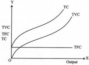
For the TC curve, the following points can be noted:

Q9) Explain properties of isoquants?

A9)

The term “iso-quants” is derived from Greek word iso means “equal” and quants means “quantity”. Thus, iso-quant means equal quantity. An iso-quant is also known as iso-production curve, iso-indifference, equal production curve by various economists. The isoquants have its properties which are similar to those generally assumed for indifference curve theory of the theory  of consumer’s behaviour analysis. Iso-quant is defined as “a locus of all the combination of two factors of production that yields that yield the same level of output.”

Thus, an iso-quant is a combination of any two factor inputs that represents and produce the same level of output. Any two combinations of input factors e.g. Labour and capital are used in which one factor is increased by decreasing the other factor of input to maintain the same level of production.

Iso-quant can be explained with the schedule and graph given below:

Factor combinations to produce a given level of output

The above table shows the five combination of inputs i.e. Labour and Factor unit which yield the same level of output of 500 units. Which says any point on the iso-quant will give the same level of output. To show this we draw the iso-quant drawn below:

Iso-quant map:

An iso-quant map represents a set of iso-quant curves shows the combination of input factor at the various level of output. A higher level of iso-quant represents the higher level of output. Thus, in simple word, iso-quant map is a family of iso-quant representing the various iso-quant curve at a particular level of output. The iso-quant map can be represented with the diagram given below:

The fig above shows the various iso-quants representing the various level of output at different combination of input factors. IQ1 , IQ2 and IQ3 shows the iso-quant which produces 100,200 and 300 units of output respectively with the various combination of input factors which provides the same level of output at different level of Iso-quant.as we had said higher the Iso-quant represents higher the value of output.

Properties

Thus, the iso-quant can be downward sloping from left to right. There can’t be an upward sloping iso-quant curve because it shows that a given product can be produce by using less of both the input factor. Similarly, an iso-quant cannot be horizontal or vertical because it also doesn’t represent the equilibrium position of a firm. Only the downward sloping supply curve represents the characteristics of iso-quant.

2.        Iso-quant are convex to the origin: As we had discussed in the above property that the iso-quant curve is downward sloping and it has a negative slope and it operates under law of Marginal rate of Technical Substitution (MRTS). It says that it equals the ratio of the marginal product if labour and marginal product of capital i.e. one factor is given up to get one additional unit of other factor to produce the same of output which creates a convexity of iso-quant curve.

Thus, the slope of iso-quant can be represented by,

The above equation represents ratio of change in capital and labour should be equal to the ratio of the marginal rate of technical substitution of labour and capital which is equal to the ratio of marginal product of labour and capital.

The convexity of iso-quant means that as we move down the curve less and less of capital given up for an additional unit of labour so to produce the same level of output. The convexity of isoquant can be observed from the diagram Given below

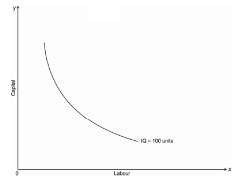
Thus, the iso-quant can be convex to the origin but not the concave because it would mean that MRTS will increase instead of decreasing i.e. labour will increase at a constant rate the amount of capital given up will goes on increasing

3.        Iso-quants do not intersect: The properties of iso-quants say that two iso-quant will never intersect each other. To explain this, we will take a help of following Diagram

The above fig represents two different iso-quant IQ1and IQ2, where it represents the level of output 100 and 200 units respectively. Point a represents 100 units of output on IQ1 and point c represents 200 units of output on IQ2. The point b shows the intersection of both the iso-quants where is logically not possible to identify the level of output.

4.        Iso-quant cannot touch either of the axis: an iso-quant cannot only touch x axis or y axis or any either axis because it will represent that the iso-quant only produce goods by using one factors of production either by using only capital or only labour which is practically not possible and which is unrealistic.

5.        Higher the iso-quant higher the level of production: if there is a multiple iso-quant showing different level of production in one diagram. Where the higher the iso-quant i.e. the iso-quant far from the origin indicates higher level of output and the iso-quant close to the origin indicates lower level of output.

Q10) Explain marginal rate of technical substitution and economic region of production?

A10)

Marginal rate of technical substitution

Marginal rate of technical substitution refers to rate, at which one

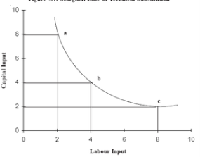
Input can be substituted for another input, without affecting the total output. Capital and labour are two inputs, in case amount of capital that can be replaced by an extra unit of labour, keeping the output constant.

Marginal rate of technical substitution of labour for capital = slope = ∆K/∆L

.

Capital and labour are not perfect substitutes for each other so The MRTS has decreased. Therefore , while keeping the output level constant, more of labour is added, less  of capital can be used.

Since, by definition, output remains constant on an isoquant the loss in physical output from a small reduction in capital will be equal to the gain in physical output from a small increment in labour.

The loss in output is calculated by multiplying the marginal physical product of capital (MP) by the amount of reduction in capital. The gain in output is calculated by multiplying the marginal physical product of labour (MP by the increment in labour.

Accordingly, along an isoquant:

∆K.MPK + ∆L.MPL = 0

∆K x MPK = ∆L x MPL

∆K/∆L = MPL/MPK

But ∆K/∆L, by definition, is the marginal rate of technical substitution of labour for capital

Therefore, MRTSLK = MPL/MPK

Thus we can see that marginal rate of technical substitution of labour for capital is the ratio of marginal physical product of the two factors labour and capital.

Economic region of production

Economic region a territorial component of a country’s national economy. Economic region is characterised by specific economic-geographical status, by an economic unity, by distinctive natural and economic conditions, and by a production specialization based on territorial social division of labor.  Under capitalism, in the heat of competition economic regions form and develop spontaneously. Under socialism, based on the economic laws of socialism, the territorial division of labor develops, and economic regions form develops in a planned fashion.

In the formation of economic regions, specialization within the social territorial division of labor plays the principal role. The boundaries of a region is determined by the specialised branches action and major auxiliary facilities—the associated cooperative suppliers of raw materials, assemblies, and parts.

Economic region is also influenced by natural conditions such as the natural fertility of the soil, and the climate, the presence of large deposits of minerals.

Other factors influencing the economic region formation are administrative and political units , technical and economic conditions.

The three levels of economic regions are as follows: large (macroregions), administrative (mesoregions), and lowest-level (microregions).

Large economic regions comprise three types: Union republics, groups of Union republics, and groups of autonomous republics. The large economy determines territorial proportions of national economies. It also determines the trends in the location of productive forces throughout the national economy.

Administrative economic regions form the basis of the country’s territorial makeup. It includes the basic elements in the territorial planning and management of the national economy.

Lowest-level economic regions are low-level administrative regions that include the primary territorial elements in the classification of economic regions.

Q11) explain optimum combination resources and expansion path?

A11)

Optimal combination of resources

Optimum factors of production are explained in two methods are as follows

Formula:

Mppa = Mppb = Mppc = Mppn

Pa         Pb        Pc        Pn

Where as,

a, b, c, n are different factors of production.

Mpp is the marginal physical product.

A firm compares the Mpp / P ratios with that of another. A firm will reduce its cost by using more of those factors with a high Mpp / P ratios and less of those with a low Mpp / P ratio until they all become equal.

2.        The isoquant approach - The least cost combination of-factors is explained with the help of iso-product curves and isocosts. The optimum factors combination or the least cost combination refers to the combination of factors to produce a specific quantity of output at the lowest possible cost. The least cost combination of factors for any level of output when the iso-product curve is tangent to an isocost curve

The choice of a particular combination of factors depends on technical possibilities of production and the prices of factors used for the production of a particular product.

The prices of factors are represented by the iso-cost line. The Iso cost line is very important in determining what combination of factors the firm will choose for production

For ex,  a firm has to spend 300/-on the factors of production such as labour and capital. Price of labour is Rs. 4 per labour hour and the price of capital is Rs. 5 per machine hour. With outlay of Rs. 300, a firm can buy 75 units of labour or 60 units capital). In the below figure, OB represent 75 units of labour and OA represent 60 units of capital.

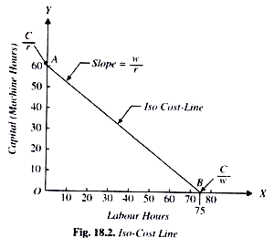
This line AB is called iso-cost line, the combination of various factors which a firm can buy with a constant out­lay. The iso-cost line is also called the price line or outlay line.

Assumption of optimum factor combination

The optimum factor combination is explained in the below diagram

The entrepreneur decides to produce 400units of output which is represented by isoquant P. The 400 unit of output can be produced by any combination of factor X(labour) and Factor Y (capital) such as R, S, Q, L and P lying on the isoquant. For producing 400 units, the cost will be minimum at point Q, which the iso-cost line CD is tangent to the given isoquant. At no other point such as R, S,L, P the cost is minimum. Therefore the firm will not choose any combination of R,S,L,P.

The expansion path

In economics, an expansion path is a line connecting optimal input combinations as the scale of production expands. A producer seeking to produce the most units of a product in the cheapest possible way to increase production along the expansion path.

Definition

Economist Alfred Stonier and Douglas Hague defined expansion path  as,” that line which reflects least cost method of producing different levels of output, when factor prices remains constant”.

Assumption

In order to maximise profits, the firm combines labour and capital in such a way that the ratio of their MP is equal to the ratio of their prices

This occurs at a point of tangency between an isocost line and an isoquant curve.

In the above figure, the different isoquant lines areC1L1,C2L2,C3L3. Keeping the prices of factors constant, the different isoquant lines are shown parallel to each other. There are three isoquants ie 100, 200, 300 representing successively higher level of output.

At point P, the firm is at equilibrium, where the isoquant 100 is tangent to its corresponding isoquant line C1L1. Similarly the firm is equilibrium at point Q and R, where the isoquant 200 and 300 is tangent to its corresponding isoquant line C2L2 and C3L3. Each point of tangency implies optimum combination of capital and labour that produces optimum level of output. The line OS joining the equilibrium point P,Q,R from the origin is the expansion path of the firm.

Q12) Explain decreasing return of scale?

A12)

Decreasing returns to scale: In this case, increase in output is less than the  increase in inputs in proportionate terms. In terms of diagram, the distance between  successive multiple isoquants increases along the product line OP as shown below :

= 20 units Q = 18 units

Q= 10 units.

Li L2 Diagram 3

At the initial combination (L1, K1) at point a on the product line OP, output is 10 units. When the factor inputs are doubled i.e., (L2 K2) at point c, the output is less than doubled i.e., Q’ = 18 units. Whereas doubling the output (Q’ = 20 units) requires more then double of the inputs. So the distance between isoquants has increased, i.e., Oa < ab, indicating decreasing return to stale.

Q13) Explain  increasing return of scale.

A13)

Increasing returns to scale. Technically, the phrase increasing returns to scale refers to the relationship between inputs and outputs. When we say that a production function exhibits increasing’returns, we mean that given percentage increase in inputs leads to a larger percentage increase in the production of output.

For example, if a firm doubled or tripled inputs, it would More than double or triple output. When the prices of inputs do not change with output levels, then the increasing.

Returns to scale also means that as output rises, average cost of production falls. In terms of the following diagram 2, increasing’returns to scale implies that the distance  between consecutive multiple isoquants decreases along the product line i.e., C a < ab.