undefined | unit 2 economy in the short run

Unit 2

Economy in the Short Run

Q1) Explain LS-LM framework.

A1)

The goods and the money markets are interlinked by two economic variables, namely: interest rate and national income. In this model, interest rate is introduced in the goods market through investment demand. The goods market therefore has two variables – interest rate (i) and national income (GDP). The goods market equation is known as the IS curve. The IS curve represents equality between saving (S) and investment (I) and all points on the IS curve show goods market equilibrium at different levels of interest and national income. The money market equilibrium is determined by the demand for and supply of money at various levels of interest and national income. The demand for money is a function of income and interest rate. The supply of money is determined by the Central Bank (the RBI in India or the Federal Reserve in the USA). The money market equation is known as the LM curve. The LM curve represents equilibrium between demand and supply of money at various levels of interest rates and national income. Various points on the LM curve shows equality between demand for money (L) and supply of money (M).

The IS-LM model shows how the equilibrium levels of income and interest rates are simultaneously determined by the simultaneous equilibrium in the two interdependent goods and money markets. Hicks, Hansen and Johnson put forward the IS-LM model on the basis of Keynesian framework of national income determination in which investment, national income, rate of interest, demand for and supply of money are interrelated and inter– dependent. These variables are represented by two curves, namely; the IS and the LM curves.

The goods market and the IS curve

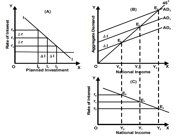
The goods market is in equilibrium when aggregate demand is equal to national income. In a closed two sector economy, the aggregate demand is determined by consumption demand and Investment demand (AD = C + I). Changes in the interest rate affect aggregate demand through changes in investment demand. With the fall in interest rates, the profitability of investment rises because the cost of investment falls. Increase in investment demand leads to increase in aggregate demand and rise in the equilibrium level of national income. The IS curve shows the different combinations of national income and interest rates at which the goods market is in equilibrium. The derivation of the IS curve is depicted in Figure given below

In panel (A) of below figure we will notice that the relationship between planned investment and rate of interest is depicted. It will be obvious from the figure that planned investment is inversely related to the rate of interest. When the interest rate falls, planned investment rises, leading to an upward shift in the aggregate demand function. The shift in the aggregate demand function is depicted in panel (B) of the figure, where in, you will see that an upward shift caused in the aggregate demand function leads to a higher level of national income in the goods market. Thus in the goods market, the level of national income is inter-connected with the interest rate through planned investment. The IS curve is the locus of various combinations of interest rates and the levels of national income at which the goods market is in equilibrium.

In panel (C) of Fig., the IS curve is depicted. It shows that the changes in the level of national income are a function of changes in the level of aggregate demand, planned investment and rate of interest. At the given rate of interest r0, the level of national income Y0 is plotted. When the interest rate falls to r1, planned investment increases to I1 and the aggregate demand function shifts from AD0 to AD1 and the goods market assumes equilibrium at Y1 level of national income. We therefore plot Y1 level of national income corresponding to r1 level of interest rate. Similarly when the interest rate further falls to r2, planned investment increases to I2 and the aggregate demand curve shifts upward to AD2. Now the goods market assumes equilibrium at Y2 level of national income. In panel (C), the equilibrium national income Y2 is shown against the rate of interest r2. By repeating this process for all possible interest rates, we can trace a series of combinations of interest rates and income levels corresponding to goods market equilibrium. By joining points such as E0, E1, E2 etc. in panel (C) of the diagram, we obtain the IS curve. You will notice that the IS curve so obtained is downward sloping indicating that when the rate of interest falls, the equilibrium national income rises.

The slope of IS curve

The IS curve has a negative slope indicating an inverse relationship between the rate of interest and the level of aggregate demand. A higher interest rate will lower the level of planned investment and hence lower the level of aggregate demand and the equilibrium level of national income. Similarly, a lower interest rate will raise the level of planned investment and hence higher will be the level of aggregate demand and the equilibrium level of national income.

The steepness of the IS curve is determined by the elasticity of investment demand curve and the size of the investment multiplier. The elasticity of investment demand shows the degree of responsiveness of investment expenditure to the changes in the rate of interest. If the investment demand is relatively elastic, a given fall in the rate of interest will result in a more than proportionate change in investment demand bringing about a larger shift in the aggregate demand curve and larger level of national income, thus making the IS curve flatter. Conversely, if the investment demand is relatively inelastic, the IS curve will be relatively steep. The steepness of the IS curve is also determined by the size of the investment multiplier. The value of the multiplier is determined by the size of the marginal propensity to consume. Greater the mpc (marginal propensity to consume), greater will be the size of the investment multiplier and greater will be the level of national income as a result of increase in investment. Thus making the IS curve flatter. Conversely, if the mpc is lower, the IS curve will have a steeper slope.

Shifts in the IS curve

Changes in autonomous expenditure causes a shift in the IS curve. Autonomous expenditure is independent of the level of income and the rate of interest. Autonomous expenditure may increase on account of increase in government expenditure, increase in autonomous consumption expenditure or increase in autonomous investment demand. Autonomous investment demand may rise due to increase in firm’s optimism about future profits. Autonomous consumption demand may rise due to households’ estimate of future incomes. Government expenditure has an autonomous component given the wide-scale use of deficit financing. An increase in autonomous expenditure at a given interest rate would shift the aggregate demand curve upwards leading to an increase in the equilibrium level of national income. With interest rate remaining constant, an upward shift in the aggregate demand curve will cause the IS curve to shift towards the right indicating increase in national income at the given interest rate.

In figure below, the shift in the IS curve is depicted by introducing the third component of the aggregate demand namely government expenditure and it is denoted by ‘G’.

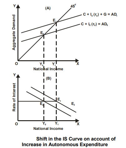
From the figure we will notice that that when the rate of interest is r0, the planned investment is I0 and the Aggregate Demand Curve is AD which intersects the 45o line at point E0 and Y0 level of national income is determined. It is also depicted in panel (B) of the diagram by point E0. Let us now introduce the government component in the composition of the aggregate demand and assume that the entire component is autonomous in nature. Government expenditure ‘G’ will shift the aggregate demand curve to AD1 which intersects the 45 o line at point E1 higher level of national income Y1 is determined. Correspondingly, we obtain point E1 on panel (B) of the diagram as the new equilibrium point and accordingly Y1 level of national income is plotted. The change in the level of national income from Y0 to Y1 is not on account of any change in the interest rate and hence the IS curve shifts to the right. The new equilibrium point E1 is horizontally contiguous and to the right of point E0 indicating a shift in the IS curve.

The movement along the IS curve indicates shifts in equilibrium income caused by shifts in the aggregate demand curve as a result of changes in interest rates. A shift in the aggregate demand curve caused by any other factor other than interest rate must be represented by a shift in the IS curve.

The money market and the LM curve

Derivation of the LM Curve:

The LM curve is often derived from the Keynesian theory from its analysis of money market equilibrium. Consistent with Keynes, demand for money to hold depends upon transactions motive and speculative motive.

It is the money held for transactions motive which is a function of income. The greater the level of income, the greater the amount of money held for transactions motive and therefore higher the extent of cash demand curve.

The demand for money depends on the extent of income because they need to finance their expenditure, that is, their transactions of shopping for goods and services. The demand for money also depends on the speed of interest which is that the cost of holding money. This is often because by holding money rather than lending it and buying other financial assets, one has to forgo interest.

Thus demand for money (Md) is expressed as:

Md – L(Y, r)

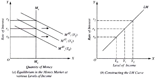
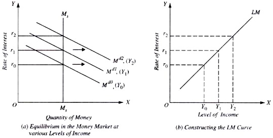
Where Md stands for demand for money, Y for real income and r for rate of interest Thus, we can draw a family of money demand curves at various levels of income. Now, the intersection of those various money demand curves like different income levels with the supply curve of money fixed by the monetary authority would gives us the LM curve.

The LM curve relates the extent of income with the rate of interest which is determined by money-market equilibrium like different levels of demand for money. The LM curve tells what the varied rates of interest are going to be (given the quantity of money and the family of demand curves for money) at different levels of income.

But the cash demand curve or what Keynes calls the liquidity preference curve alone cannot tell us what exactly the rate of interest will be. In Fig. (a) and (b) we've derived the LM curve from a family of demand curves for money. As income increases, money demand curve shifts outward and thus the rate of interest which equates supply of money, with demand for money rises. In Fig. (b) we measure income on the X-axis and plot the income level like the various interest rates determined at those income levels through money market equilibrium by the equality of demand for and therefore the supply of money in Fig. (a).

Slope of LM Curve:

It will be noticed from Fig. (b) that the LM curve slopes upward to the right. This is because with higher levels of income, demand curve for money (Md) is higher and consequently the money- market equilibrium, that is, the equality of the given money supply with money demand curve occurs at a better rate of interest. This implies that rate of interest varies directly with income.

It is important to understand the factors on which the slope of the LM curve depends. There are two factors on which the slope of the LM curve depends. First, the responsiveness of demand for money (i.e., liquidity preference) to the changes in income as the income increases, say from Y0 to Y1 the demand curve for money shifts from Md0 to Md1 that's , with an increase in income, demand for money would increase for being held for transactions motive, Md or L1 =f(Y).

This extra demand for money would disturb the money market equilibrium and for the equilibrium to be restored the rate of interest will rise to the extent where the given funds curve intersects the new demand curve like the higher income level.

It is worth noting that in the new equilibrium position, with the given stock of money supply, money held under the transactions motive will increase whereas the money held for speculative motive will decline.

The greater the extent to which demand for money for transactions motive increases with the rise in income, the greater the decline in the supply of money available for speculative motive and, given the demand for money for speculative motive, the higher the rise in tie rate of interest and consequently the steeper the LM curve, r = f (M2 L2) where r is that the rate of interest, M2 is the stock of money available for speculative motive and L2 is that the money demand or liquidity preference for speculative motive.

The second factor which determines the slope of the LM curve is that the elasticity or responsiveness of demand for money (i.e., liquidity preference for speculative motive) to the changes in rate of interest. The lower the elasticity of liquidity preference for speculative motive with reference to the changes in the rate of interest, the steeper is going to be the LM curve. On the opposite hand, if the elasticity of liquidity preference (money demand-function) to the changes within the rate of interest is high, the LM curve will be flatter or less steep.

Shifts within the LM Curve:

Another important thing to know about the IS-LM curve model is that what brings about shifts within the LM curve or, in other words, what determines the position of the LM curve. As seen above, a LM curve is drawn by keeping the stock or money supply fixed.

Therefore, when the money supply increases, given the money demand function, it'll lower the rate of interest at the given level of income. This is often because with income fixed, the speed of interest must fall so that demands for money for speculative and transactions motive rises to become equal to the greater money supply. This will cause the LM curve to shift outward to the right.

The other factor which causes a shift within the LM curve is the change in liquidity preference (money demand function) for a given level of income. If the liquidity preference function for a given level of income shifts upward, this, given the stock of money, will cause the rise within the rate of interest for a given level of income. This will cause a shift within the LM curve to the left.

It therefore follows from above that increase within the money demand function causes the LM curve to shift to the left. Similarly, on the contrary, if the money demand function for a given level of income declines, it'll lower the rate of interest for a given level of income and can therefore shift the LM curve to the right.

The LM Curve: The Essential Features:

From our analysis of the LM curve, we attain its following essential features:

1. The LM curve is a schedule that describes the combinations of rate of interest and level of income at which money market is in equilibrium.

2. The LM curve slopes upward to the right.

3. The LM curve is flatter if the interest elasticity of demand for money is high. On the contrary, the LM curve is steep if the interest elasticity demand for money is low.

4. The LM curve shifts to the right when the stock of money supply is increased and it shifts to the left if the stock of money supply is reduced.

5. The LM curve shifts to the left if there's an increase within the money demand function which raises the quantity of cash demanded at the given rate of interest and income level. On the opposite hand, the LM curve shifts to the proper if there's a decrease within the money demand function which lowers the amount of money demanded at given levels of rate of interest and income.

Simultaneous Equilibrium of the goods Market and Money Market:

The IS and therefore the LM curves relate the 2 variables:

(a) Income and

(b) The rate of interest.

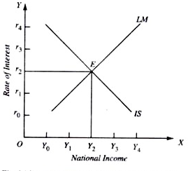
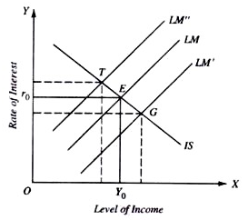
Income and therefore the rate of interest are therefore determined together at the point of intersection of those two curves, i.e., E in Fig. The equilibrium rate of interest thus determined is Or2 and therefore the level of income determined is OY2. At now income and the rate of interest stand in relation to each other such (1) the goods market is in equilibrium, that is, the aggregate demand equals the extent of aggregate output, and (2) the demand for money is in equilibrium with the supply of money (i.e., the desired amount of money is equal to the actual supply of money). It should be noted that LM cur/e has been drawn by keeping the supply of money fixed. Thus, the IS-LM curve model is predicated on:

(1) The investment-demand function,

(2) The consumption function,

(3) The money demand function, and

(4) The quantity of money.

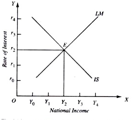
We see, therefore, that consistent with the IS-LM curve model both the real factors, namely, saving and investment, productivity of capital and propensity to consume and save, and the monetary factors, that is, the demand for money (liquidity preference) and supply of money play a part within the joint determination of the rate of interest and therefore the level of income. Any change in these factors will cause a shift in IS or LM curve and can therefore change the equilibrium levels of the rate of interest and income.

The IS-LM curve model explained above has succeeded in integrating the theory of money with the theory of income determination. And by doing so, as we shall see below, it's succeeded in synthesising the monetary and monetary policies. Further, with the IS-LM curve analysis, we are better ready to explain the effect of changes in certain important economic variables like desire to save, the supply of money, investment, demand for money on the rate of interest and level of income.

Effect of Changes in Supply of money on the rate of Interest and Income Level:

Let us first consider what will happen if the supply of money is increased by the action of the central bank. Given the liquidity preference schedule, with the increase within the supply of money, more money will be available for speculative motive at a given level of income which can cause the rate of interest to fall. As a result, the LM curve will shift to the right. With this rightward shift within the LM curve, within the new equilibrium position, rate of interest are going to be lower and therefore the level of income greater than before. This is often shown in Fig. 24.4 where with a given supply of money, LM and IS curves intersecting at point E.

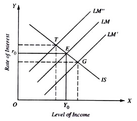
With the increase within the supply of money, LM curve shifts to the right to the position LM’, and with IS schedule remaining unchanged, new equilibrium is at point G like which rate of interest is lower and level of income greater than at E. Now, suppose that rather than increasing the supply of money, central bank of the country takes steps to reduce the supply of money.

With the reduction within the supply of money, less money will be available for speculative motive at each level of income and, as a result, the LM curve will shift to the left of E, and therefore the IS curve remaining un-changed, within the new equilibrium position (as shown by point T in Fig) the rate of interest will be higher and therefore the level of income smaller than before.

Changes in the Desire to save or Propensity to Consume:

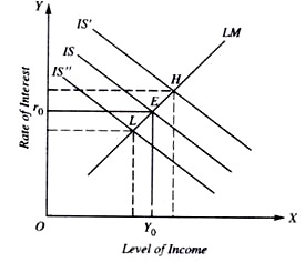
Let us consider what happens to the rate of interest when desire to save or in other words, propensity to consume changes. When people’s desire to save falls, that is, when propensity to consume rises, the aggregate demand curve will shift upward and, therefore, level of national income will rise at each rate of interest. As a result, the IS curve will shift outward to the right. In Fig. 24.5 suppose with a particular given fall within the desire to save (or increase within the propensity to consume), the IS curve shifts rightward to the dotted position IS’. With LM curve remaining unchanged, the new equilibrium position will be established at H corresponding to which rate of interest also as level of income will be greater than at E.

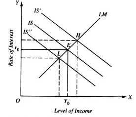
Thus, a fall within the desire to save has led to the increase in both rate of interest and level of income. On the opposite hand, if the desire to save rises, that is, if the propensity to consume falls, aggregate demand curve will shift downward which will cause the level of national income to fall for each rate of interest and as a result the IS curve will shift to the left.

With this, and LM curve remaining unchanged, the new equilibrium position will be reached to the left of E, say at point L (as shown in Fig. ) like which both rate of interest and level of national income will be smaller than at E.

Changes in Autonomous Investment and Government Expenditure:

Changes in autonomous investment and Government expenditure also will shift the IS curve. If either there's increase in autonomous private investment or Government steps up its expenditure, aggregate demand for goods will increase and this may bring about increase in national income through the multiplier process.

This will shift IS schedule to the right, and given the LM curve, the rate of interest also as the level of income will rise. On the contrary, if somehow private investment expenditure falls or the govt reduces its expenditure, the IS curve will shift to the left and, given the LM curve, both the rate of interest and therefore the level of income will fall.

Changes in Demand for Money or Liquidity Preference:

Changes in liquidity preference will bring about changes within the LM curve. If the liquidity preference or demand for money of the people rises, the LM curve will shift to the left. This is often because, greater demand for money, given the supply of money, will raise the rate of interest like each level of national income. With the leftward shift within the LM curve, given the IS curve, the equilibrium rate of interest will rise and the level of national income will fall.

On the contrary, if the demand for money or liquidity preference of the people falls, the LM curve will shift to the right. this is often because, given the supply of money, the rightward shift within the money demand curve means like each level of income there'll be lower rate of interest. With rightward shift within the LM curve, given the IS curve, the equilibrium level of rate of interest will fall and therefore the equilibrium level of national income will increase.

We thus see that changes in propensity to consume (or desire to save), autonomous investment or Government expenditure, the supply of money and therefore the demand for money will cause shifts in either IS or LM curve and can thereby bring about changes within the rate of interest also as in national income.

The integration of goods market and money market within the IS-LM curve model clearly shows that Government can influence the economic activity or the level of national income through monetary and fiscal measures.

Through adopting an appropriate monetary policy (i.e., changing the availability of money) the govt can shift the LM curve and thru pursuing an appropriate fiscal policy (expenditure and taxation policy) the govt can shift the IS curve. Thus both monetary and fiscal policies can play a useful role in regulating the extent of economic activity within the country.

Critique of the IS-LM Curve Model:

The IS-LM curve model makes a major advance in explaining the simultaneous determination of the rate of interest and therefore the level of national income. It represents a more general, inclusive and realistic approach to the determination of interest rate and level of income.

Further, the IS-LM model succeeds in integrating and synthesising fiscal with monetary policies, and theory of income determination with the theory of money. But the IS-LM curve model isn't without limitations.

Firstly, it's based on the assumption that the rate of interest is quite flexible, that is, free to vary and not rigidly fixed by the financial institution of a country. If the rate of interest is sort of inflexible, then the appropriate adjustment explained above will not take place.

Secondly, the model is additionally based upon the assumption that investment is interest-elastic, that is, investment varies with the rate of interest. If investment is interest-inelastic, then the IS-LM curve model breaks down since the required adjustments do not occur.

Thirdly, Don Patinkin and Friedman have criticised the IS-LM curve model as being too, artificial and over-simplified. In their view, division of the economy into two sectors – monetary and real – is artificial and unrealistic. According to them, monetary and real sectors are quite interwoven and act and react on one another.

Further, Patinkin has acknowledged that the IS-LM curve model has ignored the possibility of changes within the price level of commodities. according to him, the varied economic variables like supply of money, propensity to consume or save, investment and therefore the demand for money not only influence the rate of interest and the level of national income but also the prices of commodities and services.

Potemkin has suggested a more integrated and general equilibrium approach which involves the simultaneous determination of not only the rate of interest and therefore the level of income but also of the prices of commodities and services.

Q2) Explain monetary policy.

A2)

Meaning

Monetary policy is the process of drafting, announcing, and implementing the plan of actions taken by the central bank, currency board, or other competent monetary authority of a country that controls the quantity of money in an economy and the channels by which new money is supplied.

Monetary policy aims at meeting macroeconomics objectives such as controlling inflation, consumption, growth, and liquidity which consist of the management of money supply and interest rates. This is achieved by actions such as modifying the interest rate, buying or selling government bonds, regulating foreign exchange (forex) rates, and changing the amount of money banks are required to maintain as reserves.

Definition

Monetary policy, the demand side of economic policy, refers to the actions undertaken by a nation's central bank to control money supply and achieve macroeconomic goals that promote sustainable economic growth.

Johnson defines monetary policy “as policy employing central bank’s control of the supply of money as an instrument for achieving the objectives of general economic policy.”

G.K. Shaw defines it as “any conscious action undertaken by the monetary authorities to change the quantity, availability or cost of money.”

Objectives

Full employment - The foremost objectives of monetary policy is full employment. It is an important goal not only because unemployment leads to wastage of potential output, but also because of the loss of social standing and self-respect.

2. Price stability – One of the objectives of monetary policy is to stabilize the price level. This policy is favored because fluctuations in prices bring uncertainty and instability to the economy.

3. Economic growth – In the recent years the most important objectives of monetary policy has been the rapid economic growth of an economy. Economic growth is defined as “the process whereby the real per capita income of a country increases over a long period of time.”

4. Balance of payment – Many developing countries like India suffers from the Disequilibrium in the BOP. The Reserve Bank of India through its monetary policy tries to maintain equilibrium in the balance of payments. The BOP has two aspects i.e. the 'BOP Surplus' and the 'BOP Deficit'. The former reflects an excess money supply in the domestic economy, while the later stands for stringency of money. If the monetary policy succeeds in maintaining monetary equilibrium, then the BOP equilibrium can be achieved.

5. Exchange Rate Stability: Exchange rate is the price of a home currency expressed in terms of any foreign currency. If this exchange rate is very volatile leading to frequent ups and downs in the exchange rate, the international community might lose confidence in our economy. The monetary policy aims at maintaining the relative stability in the exchange rate. The RBI by altering the foreign exchange reserves tries to influence the demand for foreign exchange and tries to maintain the exchange rate stability.

6. Neutrality of Money: Economist such as Wicksted, Robertson have always considered money as a passive factor. According to them, money should play only a role of medium of exchange and not more than that. Therefore, the monetary policy should regulate the supply of money. The change in money supply creates monetary disequilibrium. Thus monetary policy has to regulate the supply of money and neutralize the effect of money expansion. However this objective of a monetary policy is always criticized on the ground that if money supply is kept constant then it would be difficult to attain price stability.

Instruments of monetary policy

Bank rate policy – The minimum lending rate is the bank rate of the central bank at which it rediscounts first class bills of exchange and government securities held by the commercial banks. Central banks raise the bank rate when it finds that inflationary pressures have started emerging within the economy. Commercial bank borrows less as borrowing from central bank become costly. In turn, commercial banks raise their lending rate to the business community and the borrowers borrow less from commercial bank.

On the other hand central banks lower the bank rate when prices are depressed. On the part of commercial bank it is cheap to borrow from the central bank. The commercial bank lowers their lending rate and encourages business men to borrow more.

2. Open market operation – Open market operations refer to sale and purchase of securities in the money market by the central bank. The central bank sells securities, when prices are rising and there is need to control them. The reserves of commercial banks are reduced and they are not in a position to lend more to the business community.

On the contrary, the central bank buys securities, when recessionary forces start in the economy. The commercial bank reserves are raised and they lend more to the business community.

3. Changes in reserves ratio – Every bank is required to keep certain percentage of its total deposits with the central bank. The central bank raise the reserve ratio when prices are rising. Banks are required to keep more with the central bank. Their reserves are reduced and they lend less. In the opposite case, the reserves of commercial banks are raised, when the reserve ratio is lowered. They lend more and the economic activity is favorably affected.

4. Selective credit controls - For particular purposes selective credit controls are used to influence specific types of credit. The central bank raises the margin requirement when there is brisk speculative activity in the economy or in particular sectors in certain commodities and prices start rising. The result is that the borrowers are given less money in loans against specified securities. In case of recession in a particular sector, the central bank encourages borrowing by lowering margin requirements.

Q3) Explain fiscal policy.

A3)

Fiscal Policy refers to the methods employed by the government to influence and monitor the economy by adjusting taxes and/or public spending. In doing so, the government aims to find a balance between lowering unemployment and reducing the inflation rate. The main tools of Fiscal Policy are changes in the composition of taxation and government spending.

Definitions

“By fiscal policy we denote to government actions afflicting its receipts and outlays which are ordinarily taken as measured by the government’s receipts, its surplus or deficit.”

“A policy under which the government uses its outlay and revenue programmes to produce desirable effects and avoid undesirable effects on the national earnings, manufacturing and employment.”

Objectives of fiscal policy-

1. To uphold and accomplish full employment.

2. To alleviate the price level.

3. To soothe the development rate of financial system.

4. To sustain symmetry in the balance of payment.

5. To endorse the monetary development of under developed nations.

Instruments of Fiscal Policy

Following are the main instruments of fiscal policy:

Public Expenditure- Public Expenditure means expenditure incurred by the government of a country. It generates sufficient influence on aggregate demand and development activities of a country. The expenditure can be of two types:

Expenditure incurred by the government to get goods and services. It directly influences aggregate demand.
Public expenditure incurred on pensions, scholarships, educational and medical facilities to people etc. This expenditure is known as Transfer Payment. It also raises aggregate demand.

Modern states are welfare oriented states and they have to use money to achieve this end. Tax is the main source to acquire money. Aggregate demand can also be influenced by taxes. Government collects money by imposing different taxes to finance public expenditure and to manage various development activities. Mainly, taxes can be classified into two groups

Direct Tax: Direct tax reduces the income of the people and a part of their income goes into the government treasury.
Indirect Tax: Indirect taxes lead to a rise in prices of goods.

3. Public Debt: The third instrument of fiscal policy is public debt. Public debt means debt taken by the government from people or from the governments of other countries. The government has to take the help of public debt if public expenditure exceeds public revenue. Public debt can be of two types: Internal and External.

4. Deficit Financing: A public expenditure has to be incurred for economic development. This amount can be collected only through the public debt, taxation etc. So deficit financing has to be introduced. When there emerges a deficit due to excess of public expenditure over public revenue, this deficit is met with either by borrowing from the central bank or by issuing new notes. Deficit financing can be used to meet government expenditure. It increases aggregate demand.

Q4) Explain shift in aggregate demand.

A4)

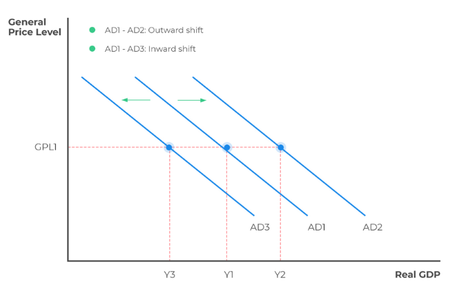
Price and other factors influencing the level of expenditure by households, governments, firms, and foreigners will cause a shift in the aggregate demand curve.

Those factors include:

Household Wealth

Household wealth incorporates both financial and real assets. Households save part of their income to accumulate wealth. With assets increasing in value, they will be forced to save less and increase spending, thus shift the aggregate demand curve to the right. Conversely, a decrease in wealth reduces consumer spending and shifts the aggregate demand curve left. This is commonly called by economists the wealth effect.

Consumer and Business Expectations

When consumers have higher confidence in staying out of unemployment, they tend to consume more, thus shifting the aggregate demand curve to the right. However, when consumers lack confidence, spending declines, shifting the AD curve to the left. For example, in the US, AIM’s Business Confidence Index is a widely followed economic indicator used by employers, traders, and governments to gauge the sentiment of consumers.

Capacity Utilization

Capacity utilization is a measure of how the economy’s production capacity is fully utilized. Businesses running below full capacity are often willing to increase their investment spending during economically good times. This makes the aggregate demand curve shift rightward.

Fiscal Policy

Fiscal policy refers to the use of taxes and government spending to affect the level of aggregate expenditure. The rise in government expenditure shifts the aggregate demand curve rightward, while a reduction in government expenditure shifts the curve to the left. This can be seen in almost every country, but most notably in the US, where infrastructure spending has been a top priority for governments in the last decade. The bet that the governments are making is that keeping people employed will have them spend more and subsequently stimulate the economy.

Low taxes lead to a high proportion of personal income and corporate pre-tax profits, and thus the individual consumers and the business entities have more to spend, shifting the AD curve to the right. On the other hand, high taxes will shift AD to the left.

Monetary Policy

Monetary policy refers to the method by a country’s central bank to alter aggregate output and prices by changing bank reserves and reserve requirements. Central banks, through various monetary policies, control the money supply. An increase in the money supply causes a rightward shift in the aggregate demand curve, whereas a reduction in the money supply shifts the aggregate demand curve leftward.

Growth in the Global Economy

Through international trade, countries are connected to form a global economy. A rapid growth in a foreign country encourages foreigners to buy more products from the domestic country, increasing the exports of the domestic country. This, in turn, shifts the AD of the domestic country to the right. This will also imply that a decline in the growth rate in the exporting country will affect the AD of the importing country.

Change in Exchange Rates

An exchange rate refers to the price of one currency in relation to another. Changes in exchange rates affect the prices of exports and imports, which is translated to AD. For example, a lower Canadian Dollar in relation to other currencies makes Canadian exports cheaper and foreign products sold in Canada expensive, shifting the AD curve of Canada to the right and vice versa.

Q5) Explain aggregate supply in short and long run.

A5)

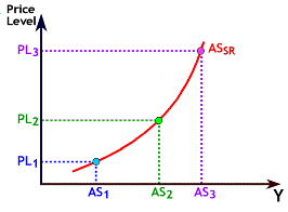
The Aggregate Supply curve graphs the total amount of output (Y) produced at various price levels. A significant difference exists between the short-run Aggregate Supply curve and the long-run Aggregate Supply curve. In the short run the Aggregate Supply curve is upward sloping. In the long run the Aggregate Supply curve is vertical.

In the context of the Aggregate Supply curve, the short run is a time period in which the costs of production--wages, raw materials, energy, and so on--are held constant; only output prices vary. When prices rise, the level of Aggregate Supply also rises because firms seek to take advantage of the profit opportunities. A firm's profit is the difference between its revenues and costs over a given time period, say one year. Suppose that a firm produces picture frames and it uses only one input, labor. Each picture frame requires one labor hour to produce, and wages are Rs 8 per hour. The firm sells each picture frame for Rs 10 so the profit per picture frame is Rs 2 (Rs 10 - Rs 8). If the firm sells 2,000 picture frames in the first year, its total profit is Rs 4,000 (2,000 x Rs 2). In the second year, the firm increases the price per picture frame to Rs 11. By assumption, wages are unchanged at Rs 8 per hour. The firm's profit per frame produced is $3. The chance for the firm to increase its profits provides an incentive for the firm to increase production. By producing and selling 2,500 picture frames in the second year, the firm's profits rise to Rs 7,500 (2,500 x Rs 3). An increase in the price level, therefore, leads to a short run increase in Aggregate Supply. The Figure labeled "Short Run Aggregate Supply Curve" is upward sloping, which illustrates the positive relationship between the price level and Aggregate Supply.

We define the long run as a time period in which all prices and costs are variable. An increase in the price level will have no impact on Aggregate Supply in the long run because all firms' costs (e.g. wages and resource costs) will rise proportionally with the price level. Recall that the picture frame company increased profits by increasing the price of picture frames from Rs 10 to Rs 11. Over time, workers adjust their wage demands upward because goods and services are more expensive and because good workers are harder to find as employment rises with the level of production. Suppose that workers increase their wage demands to Rs 9 per hour. Now the firm earns the same Rs 2 profit per frame as it did before the price level increase and the level of output returns to 2,000, the same level of production as in the first year. In the long run, the Aggregate Supply curve is vertical as illustrated in the Figure labeled "Long Run Aggregate Supply Curve." When resources such as labor and capital are fully employed, the economy's production is at the potential level of output, Yp. When the economy is on the Long Run Aggregate Supply curve, GDP is equal to potential output.

Q6) Explain determinants of aggregate demand.

A6)

Aggregate demand refers to the total demand for final goods and services in an economy during an accounting year. Aggregate demand is the sum of four components: consumption, investment, government spending, and net exports.

Consumption can change for a number of reasons, including movements in income, taxes, expectations about future income, and changes in wealth levels.

Investment can change in response to its expected profitability, which in turn is shaped by expectations about future economic growth, the creation of new technologies, the price of key inputs, and tax incentives for investment. Investment can also change when interest rates rise or fall.

Government spending and taxes are determined by political considerations.

Exports and imports change according to relative growth rates and prices between two economies.

What determines consumption expenditure?

Consumption expenditure is spending by households and individuals on durable goods, nondurable goods, and services. Durable goods are things that last and provide value over time, such as automobiles. Nondurable goods are things like groceries—once you consume them, they are gone. Services are intangible things consumers buy, like healthcare or entertainment.

Keynes identified three factors that affect consumption:

Disposable income: For most people, the single most powerful determinant of how much they consume is how much income they have in their take-home pay. This left-over income is also also known as disposable income, which is income after taxes.

Expected future income: Consumer expectations about future income also are important in determining consumption. If consumers feel optimistic about the future, they are more likely to spend and increase overall aggregate demand. News of recession and troubles in the economy will make them pull back on consumption.

Wealth or credit: When households experience a rise in wealth, they may be willing to consume a higher share of their income and to save less. When the US stock market rose dramatically in the late 1990s, for example, US rates of saving declined, probably in part because people felt that their wealth had increased and there was less need to save. How do people spend beyond their income when they perceive their wealth increasing? The answer is borrowing. On the other side, when the US stock market declined about 40% from March 2008 to March 2009, people felt far greater uncertainty about their economic future, so rates of saving increased while consumption declined.

Finally, Keynes noted that a variety of other factors combine to determine how much people save and spend. If household preferences about saving shift in a way that encourages consumption rather than saving, then aggregate demand will shift out to the right.

What determines investment expenditure?

Spending on new capital goods is called investment expenditure. Investment falls into four categories: producer’s durable equipment and software, new nonresidential structures, changes in inventories, and residential structures. The first three types of investment are conducted by businesses, while the last is conducted by households.

Keynes’s treatment of investment focuses on the key role of expectations about the future in influencing business decisions.

When a business decides to make an investment in physical assets—like plants or equipment—or in intangible assets—like skills or a research and development project—that firm considers both the expected benefits of the investment, like future profits, and the costs of the investment, such as interest rates.

The clearest driver of the benefits of an investment is expectations for future profits. When an economy is expected to grow, businesses perceive a growing market for their products. Their higher degree of business confidence will encourage new investment. For example, in the second half of the 1990s, US investment levels surged from 18% of GDP in 1994 to 21% in 2000. However, when a recession started in 2001, US investment levels quickly sank back to 18% of GDP by 2002.

Interest rates also play a significant role in determining how much investment a firm will make. Just as individuals need to borrow money to purchase homes, businesses need financing when they purchase big ticket items. The cost of investment thus includes the interest rate. Even if the firm has the funds, the interest rate measures the opportunity cost of purchasing business capital. Lower interest rates stimulate investment spending and higher interest rates reduce it.

Many factors can affect the expected profitability on investment. For example, if the price of energy declines, then investments that use energy as an input will yield higher profits. If the government offers special incentives for investment—for example, through the tax code—then investment will look more attractive; conversely, if government removes special investment incentives from the tax code or increases other business taxes, then investment will look less attractive.

Keynes believed that business investment is the most variable of all the components of aggregate demand.

What determines government spending?

The third component of aggregate demand is spending by federal, state, and local governments. Although the United States is usually thought of as a market economy, government still plays a significant role in the economy. Government provides important public services such as national defense, transportation infrastructure, and education.

Keynes recognized that the government budget offered a powerful tool for influencing aggregate demand. Not only could aggregate demand be stimulated by more government spending—or reduced by less government spending—but consumption and investment spending could be influenced by lowering or raising tax rates.

Keynes concluded that during extreme times like deep recessions, only the government had the power and resources to move aggregate demand.

What determines net exports?

Exports are products produced domestically and sold abroad, and imports are products produced abroad but purchased domestically. Since aggregate demand is defined as spending on domestic goods and services, export expenditures add to aggregate demand, while import expenditures subtract from aggregate demand.

Two sets of factors can cause shifts in export and import demand: changes in relative growth rates between countries and changes in relative prices between countries.

The level of demand for a nation’s exports tends to be most heavily affected by what is happening in the economies of the countries that would be purchasing those exports. For example, if major importers of US-made products like Canada, Japan, and Germany have recessions, exports of US products to those countries are likely to decline since quantity of a nation’s imports is directly affected by the amount of income in the domestic economy. More income will bring a higher level of imports.

Exports and imports can also be affected by relative prices of goods in domestic and international markets. If US goods are relatively cheaper compared with goods made in other places—perhaps because a group of US producers has mastered certain productivity breakthroughs—then US exports are likely to rise. If US goods become relatively more expensive—perhaps because a change in the exchange rate between the US dollar and other currencies has pushed up the price of inputs to production in the United States—then exports from US producers are likely to decline.

Q7) Explain aggregate demand and supply analysis.

A7)

Aggregate Demand (AD):

Aggregate demand is the total of all demands or expenditures within the economy at any given price over a given period time. It is therefore a quantitative sum of all the individual demands (quantity that is bought at any given price) within the economy. In economics ‘aggregate’ refers to the ‘total’ or ‘added up amount’.

Aggregate demand is also different from individual demand that it is composed from four different components, which are: consumption (C), investment (I), government spending (G) and exports minus imports (X-M). Hence, it can be represented by the formula:

AD = C I G ( X – M )

Consumption refers to the spending by households on goods and services and may also be cited as consumer spending under some circumstances. The meaning of investment is also very specific in that it refers to the spending by firms on investment goods and is not the general purchase of capital goods within the economy. Government spending also specifically includes current spending for on wages and salaries and the spending by government on investment goods such as new roads, schools and hospitals. The final component is exports less imports as when foreigners spend on domestic goods they add to the national expenditure on the local economy. On the other hand, when the local population spends on foreign goods, this is a withdrawal from the economy and effectively has the effect of reducing the national output, hence not contributing to the national income of the economy. It is important to note that all the three components of consumption, investment, government spending may also include spending on imports, thus these should be taken into account when deducting from the aggregate demand figure.

The components of aggregate demand all have different weightings, as a result, the effect of changes in some components are more significant than the changes in other components. The most significant component is considered to be consumption, as in the UK household spending accounts for over sixty five percent of aggregate demand. This might be because consumer spending is controlled by the general population in the economy which is the largest economic group in the UK. Alternatively, capital investment spending by firms in the UK accounts for 15-20% of GDP in any given year. Most of this investment, at a rate of 75% comes from private sector businesses such as Tesco and British Airways while the rest is due to public sector spending such as spending on the improvement of the healthcare. It should be appreciated that public sector spending falls under business investment and not government spending which is solely on state-provided goods and services, including public and merit goods. Government spending can be considered to be the most variable of aggregate demand as decisions on annual government spending are based the development of the economy and changing political priorities. In an average year the government accounts for about 20% of GDP in the economy. Furthermore, transfer payments in the form of welfare benefits are also don’t fall under government spending.

Nevertheless, aggregate demand can be influenced by a range of factors. One of the most important factors that may affect aggregate demand can be considered to be taxation – both direct and indirect. A decrease in taxation is likely to cause an increase in consumption due to their being higher disposable incomes available to the government. Moreover, the decrease in indirect taxation, such as VAT is likely to make goods cheaper, therefore increasing demand for these goods. A decrease in corporation tax is also likely to cause an increase in business investment as now there are more retained profits that can be put back into the business. An increase in taxation is also likely to increase government revenue, which may lead to an increase in government spending. Thus, overall a decrease in taxation is like to cause an increase in aggregate demand and vice versa.

Interest rates may also have an effect on the levels of aggregate demand in the economy. As interest rates can be considered to be a cost of borrowing a decrease in them is likely to mean it becomes cheaper to borrow, as a result borrowing may be encouraged in the economy. Thus it is likely that business investment is likely to increase along with consumer spending as both businesses and consumers can increase their funds through borrowing. Another factor may be the level of inflation and price stability in the economy over a period of time. Low inflation will mean that there is a lower decrease in the value of savings, hence there might not be a change in disposable incomes, encouraging spending. Also, low inflation means that factors of production are available to businesses at a lower price, which may lead to higher investment by businesses. As a result, both low inflation and interest rates may lead to higher levels of aggregate demand which may also be achieved if there are high levels of availability of credit in the economy as this means that there is an easier access to cash.

The level of marginal propensity to consume and the marginal propensity to save also have an effect on the level of aggregate demand in the economy, with aggregate demand being the highest when there is a high marginal propensity to consume but it is low for savers. This is because it means that less money is withdrawn from the circulation hence leading to a larger multiplier effect which is a knock on effect from an initial economic activity. Nevertheless, there are some factors that are likely to have the largest effect on government expenditure such as political and public pressure, which could force the government to either spend or save. Moreover, a decrease in living standards and under consumption of merit goods may also cause aggregate demand to increase as it can force the government to increase their spending in order to restore living standards.

Aggregate Supply (AS):

There are two types of long run aggregate supply curves. The first figure is the Monetarist curve which may also be referred to as the classical long run aggregate supply curve. The other type of curve is called the Keynesian supply curve. The Monetarist curve is a vertical straight line showing that supply is inelastic in the long run. This is because it is based on the classical view that markets tend to correct themselves fairly quickly when they are pushed into disequilibrium by some shock. According to such a view all markets are likely to be in equilibrium, hence there are no unemployed resources in the economy as it is operating at full potential. As a result there can be no increase in supply as there are no spare factors of production available, leading to an inelastic long run aggregate supply curve.

Q8) Explain fiscal and monetary policy.

A8)

Fiscal policy and monetary policy

Monetary policy

Meaning

Definition

Johnson defines monetary policy “as policy employing central bank’s control of the supply of money as an instrument for achieving the objectives of general economic policy.”

G.K. Shaw defines it as “any conscious action undertaken by the monetary authorities to change the quantity, availability or cost of money.”

Objectives

Instruments of monetary policy

On the contrary, the central bank buys securities, when recessionary forces start in the economy. The commercial bank reserves are raised and they lend more to the business community.

Fiscal policy

Definitions

“By fiscal policy we denote to government actions afflicting its receipts and outlays which are ordinarily taken as measured by the government’s receipts, its surplus or deficit.”

“A policy under which the government uses its outlay and revenue programmes to produce desirable effects and avoid undesirable effects on the national earnings, manufacturing and employment.”

Objectives of fiscal policy-

1. To uphold and accomplish full employment.

2. To alleviate the price level.

3. To soothe the development rate of financial system.

4. To sustain symmetry in the balance of payment.

5. To endorse the monetary development of under developed nations.

Instruments of Fiscal Policy

Following are the main instruments of fiscal policy:

Expenditure incurred by the government to get goods and services. It directly influences aggregate demand.
Public expenditure incurred on pensions, scholarships, educational and medical facilities to people etc. This expenditure is known as Transfer Payment. It also raises aggregate demand.

Direct Tax: Direct tax reduces the income of the people and a part of their income goes into the government treasury.
Indirect Tax: Indirect taxes lead to a rise in prices of goods.

Q9) Explain the objectives of monetary policy.

A9)

Monetary policy

Meaning

Definition

Johnson defines monetary policy “as policy employing central bank’s control of the supply of money as an instrument for achieving the objectives of general economic policy.”

G.K. Shaw defines it as “any conscious action undertaken by the monetary authorities to change the quantity, availability or cost of money.”

Objectives

Q10) Explain the instrument of monetary policy.

A10)

Fiscal policy and monetary policy

Monetary policy

Meaning

Definition

Johnson defines monetary policy “as policy employing central bank’s control of the supply of money as an instrument for achieving the objectives of general economic policy.”

G.K. Shaw defines it as “any conscious action undertaken by the monetary authorities to change the quantity, availability or cost of money.”

Instruments of monetary policy

On the contrary, the central bank buys securities, when recessionary forces start in the economy. The commercial bank reserves are raised and they lend more to the business community.

Q11) Explain instrument of fiscal policy.

A11)

Definitions

“By fiscal policy we denote to government actions afflicting its receipts and outlays which are ordinarily taken as measured by the government’s receipts, its surplus or deficit.”

“A policy under which the government uses its outlay and revenue programmes to produce desirable effects and avoid undesirable effects on the national earnings, manufacturing and employment.”

Objectives of fiscal policy-

1. To uphold and accomplish full employment.

2. To alleviate the price level.

3. To soothe the development rate of financial system.

4. To sustain symmetry in the balance of payment.

5. To endorse the monetary development of under developed nations.

Instruments of Fiscal Policy

Following are the main instruments of fiscal policy:

Expenditure incurred by the government to get goods and services. It directly influences aggregate demand.
Public expenditure incurred on pensions, scholarships, educational and medical facilities to people etc. This expenditure is known as Transfer Payment. It also raises aggregate demand.

Direct Tax: Direct tax reduces the income of the people and a part of their income goes into the government treasury.
Indirect Tax: Indirect taxes lead to a rise in prices of goods.

Sign Up