UNIT III
Spreadsheet and its Business Applications
Q1) What is Microsoft Excel?
A1) Microsoft Excel is an electronic spreadsheet application that allows users to store, organize, calculate, and manipulate data using mathematical formulas using a spreadsheet system that is split by rows and columns. It also gives you the flexibility to use an external database for analysis, reporting, and more, saving you a lot of time.
Q2) What is a ribbon?
A2) The ribbon is the top area of the application that contains menu items and toolbars available in MS-Excel. The ribbon can be shown / hidden using CTRL + F1. The ribbon runs at the top of the application and replaces toolbars and menus. There are various tabs at the top of the ribbon, and each tab has its own command group.
Q3) Explain the spreadsheet and its basics.
A3) Spreadsheets can be compared to paper ledger sheets which consists of rows and columns, and their intersection called cells. A spreadsheet is a piece of software that allows you to quickly perform quantitative analyses on statistical data, such as totalling long columns of data or calculating percentages and averages. And if some of the raw data you enter into the spreadsheet change – for example, if you have final statistics to replace provisional ones – the spreadsheet will adjust any of the equations you've done based on the new numbers.
You may also use a spreadsheet to create data visualisations, such as maps, to show the statistical data you've gathered on a website.
Q4) How many data formats can be used in Excel? Name some of them.
A4) Microsoft Excel has 11 data formats available for data storage. Example:
Q5) Specify the order of operations used to evaluate the formula in Excel.
A5) The order of operations in Microsoft Excel is the same as standard mathematics. It is defined by the term "PEMDAS" or "BEDMAS".
Q6) How can we wrap text in a cell?
A6) You can wrap the text in a cell by selecting the text you want to wrap and then clicking Wrap Text on the Home tab.
Q70 Explain macros in MS-Excel.
A7) Macros are used to iterate over groups of tasks. Users can create customized iterative function and instruction macros. Macros can be created or recorded according to the user.
Q8) What are the two languages (macro) of MS-Excel?
A8) XLM and VBA (Visual Basic Applications). Earlier versions of Excel used XLM. VBA was introduced in Excel 5 and is currently used primarily.
Q9) How can we stop someone from copying cells from your worksheet?
A9) Yes. It is possible. To protect your worksheet from copying, you need to go to Menu Bar> Review> Sheet Protection> Password. By entering the password, you can protect the sheet from being copied by others.
Q10) What is an MS-Excel chart?
A10) Graphs are provided to allow Excel to represent the data graphically. Users can use any type of graph, including columns, bars, lines, circles, and scatter plots, by selecting an option from the Graph group on the Insert tab.
Q11) How can I quickly sum the row and column numbers in an Excel sheet?
A11) You can use the SUM function to get the row and column sums in an Excel worksheet.
Q12) Explain some useful functions of Excel.
A12) The functions you can use in Excel to work with your data are:
Q13) What does the red triangle in the upper right corner of the cell indicate?
A13) A red triangle indicates that the comment is associated with a cell. You can hover your mouse over it to read the entire comment.
Q14) How do we add a new Excel worksheet?
A14) To add a new Excel worksheet, you need to insert a worksheet tab at the bottom of the screen.
15) What is the usage of Name Box in MS-Excel?
A15) The Name box is used to enter a range name or cell address in the Name box to return to a specific area of the worksheet.
Q16) How do we resize a column?
A16) To resize a column, you need to resize one column and then drag the right border of the column heading to the desired width. Another option is to select Format from the Home tab. For Format, you must select Auto Adjust Column Width below the cell section. Click this to format the cell size.
Q17) Explains the pivot table and how to use it.
A17) Pivot tables are a tool that allows you to quickly summarize large amounts of data. Automatically sort, count, sum, or average the data stored in a spreadsheet and display the results in a separate spreadsheet. It saves a lot of time. You can link external data sources to Excel.
Q18) What are the three report formats available in Excel?
A18) The types of report formats are:
Q19) How do you provide dynamic range for the "data source" of a pivot table?
A19) To provide a dynamic range for the PivotTable's "data source", first use the offset function to create a named range and then use the named range created in the first step to base it on the PivotTable.
Q20) Is it possible to create a pivot table using multiple data sources?
A20) If multiple sources are different worksheets in the same workbook, you can use multiple data sources to create a pivot table.
Q21) Which event do you hold? Do you want to use it to see if the pivot table has changed?
A21) To see if the PivotTable has changed, use Pivot Table Update on the worksheet that contains the PivotTable.
Q22) How do I disable automatic sorting of PivotTables?
A22) To disable automatic sorting of PivotTables:
Go> Other Sort Options> Right-click PivotTable> Select Sort Menu> Select More Options> Deselect Automatic Sort.
Q23) What is MS-Excel Freeze Pane?
A23) In order to Lock rows or columns use the freeze pane. Locked rows or columns are displayed on the screen even after scrolling the sheet vertically or horizontally.
Q24) How can we prevent the PivotTable from losing column width when updating?
A24) PivotTable format loss can be stopped by simply changing the PivotTable options. Under PivotTable Options, check Enable Format Preservation and disable the AutoFormat option.
Q25) Explain the protection type of workbook in Excel.
A25) Excel has three ways to protect your workbook.
Q26) Please explain the difference between the SUBSTITUTE function and REPLACE function of MS-Excel.
A26) The SUBSTITUTE function replaces one or more instances of old text with the new text in the string.
Syntax: SUBSTITUTE (text, oldText, newText, [instanceNumber])
Example: Let the text of A2 be Guru99, Guru99
SUBSTITUTE (A2, "9", "8", 1) => Guru89, Guru99
SUBSTITUTE (A2, "9", "8", 2) => Guru88, Guru99
SUBSTITUTE (A2, "9", "9") => Guru99, Guru99
The REPLACE function exchanges part of a text string with another set of text.
Syntax: REPLACE (oldText, startNumber, NumberCharacters, newText)
Example: Let the text of A2 be Guru99
REPLACE (A2,5,1, "00") => Guru009
Q27) State the differences between COUNT, COUNTA, COUNTIF and COUNTBLANK in Ms-Excel.
A27) COUNT is used to count cells that contain numbers, dates, and so on. The value stored as a number without spaces.
COUNTA or Count All is used to count cell values, including numbers, text, logical values, and so on. All types of values except whitespace.
COUNTBLANK counts cells with blank cells or empty strings.
Count cells that match a particular criterion are COUNTIF and COUNTIFS.
Q28) What is the IF function in Excel?
A28) To run a logical test, run the IF function. If the condition is true, the result will be obtained accordingly. If the condition is false, the result or output will be different.
Example: For example, suppose you select a cell and display it as "greater than 5" if the value is true (= 5 or 5) and "less than 5" if the value is false (<5). To do this, you can use IF conditions to view the results.
= IF (logical test, value if true, value if false)
= IF (A1> 5, "greater than 5," less than 5 ")
Q29) Can we create a shortcut to an Excel function?
A29) Above the home button, the Quick Access Toolbar can be customized to display the most frequently used shortcuts. How do I create a graph between multiple worksheets / from multiple worksheets in Excel?
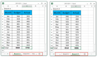
For example, four worksheets have four tables with the same layout, as shown in the screenshot below. Next, you need to extract the data series from each worksheet to create a graph, and extract the data points from each worksheet to create a graph. How can I solve them in Excel? This article recommends two workarounds:
1. Create a graph by extracting many data series from multiple worksheets
2. Extract many data points from multiple worksheets to create a graph
Extract many data series from multiple worksheets to create a graph
This section describes how to extract many data series from multiple Excel worksheets to create a column chart. You can archive by following the steps below.
1.Click Insert> Insert Column Chart (or Column)> Clustered Columns. See screenshot:
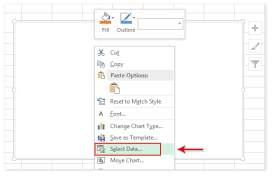
2.Insert a blank chart here. Right-click on the blank graph and select Data from the right-click menu. See screenshot:
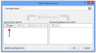
3.Open the Select Data Source dialog box and click the Add button.
4.In the Edit Series dialog box, specify the series name and series value from the worksheet and click the OK button.
5.When you return to the Select Data Source dialog box, repeat steps 3 and 4 to add data series from other worksheets. Finally, all the data series added from the worksheet are listed in the Legend Entry (Series) box, as shown in the screenshot below.
6.In the Select Data Source dialog box, click the Edit button in the Horizontal (Category) Axis Labels section to open the Axis Labels dialog box and specify the axis labels as needed. Click the [OK] button. See the screenshot above.
7.Click the OK button to close the Select Data Source dialog box
8.Optional. Continue to select the graph, click Design> Add Graph Element> Legend, and select Legend Options from the submenu. See screenshot.
In this example, select Legend> Below.
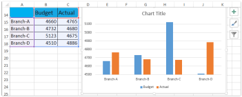
So far, you've created a clustered column chart with four data series from four worksheets. See screenshot:
Extract many data points from multiple worksheets to create a graph
You may want to create a graph whose data points are from different worksheets. This section introduces Kutools for Excel's Dynamically Browse Worksheets to extract data points from multiple worksheets into new worksheets and use these data points to create graphs.
Kutools for Excel-Includes over 300 handy tools for Excel. 30-day full-featured free trial, no credit card required! Free trial now!
1. On the Sheet tab bar, click the New button or create a new worksheet.
2. In the new worksheet, select the cell whose contents you want to extract from other worksheets and click Kutools> Other (in the Formula group)> Dynamic.
See worksheet. See screenshot:
The document dynamically references Sheet 1
3. Open the Enter Worksheet Reference dialog box and do the following:
(1) Select [Fill vertically after cell] from the [Fill order] drop-down list.
(2) In the Worksheet List section, review the worksheet from which you want to extract the data points.
(3) Click the [Fill Range] button and the [Close] button in succession.
Note: If you have multiple data series with data points from different worksheets, you can repeat this step if necessary.
Then you can see that the data points are extracted from various worksheets. See screenshot:
4. Select the extracted data points and create a graph. In this example, click Insert> Insert Column Chart (or Column)> Clustered Columns to create a clustered column.
So far, you've created a clustered column chart with data points from different worksheets. See screenshot.
Q30) What is the usage of the LOOKUP function in Excel?
A30) In Microsoft Excel, the LOOKUP function returns a value from a range or array.
Q31) How do I apply the same format to all sheets in an MS-Excel workbook?
A31) Right-click on the Worksheets tab and select All Sheets. This will apply all the formatting done to the entire workbook. To apply to a specific sheet group, select only the sheets that need to be formatted.
Q32) What are left, right, fill, and distributed placement?
A32) Left / Right Align aligns the text to the left and right of most of the cells.
As the name implies, repeat the same text in the cell.
We need to Spreads the text across the width of the cell.
left
fill
distribution
Abu
Ababa Baba Baba Bab
a b
A
aaaaaaaaaaaaaaaa
A
Q33) Which key do you press to move to the previous worksheet and the next sheet?
A33) Use Ctrl + PgUp to move to the previous worksheet and Ctrl + PgDown to move to the next sheet.
Q34) Which filter should you use if you need more than two conditions, or if you want to use the database function to analyze the list?
A34) Use advanced criteria filters to analyze the list or see if you need to test more than two conditions.
Q35) What is an easy way to get back to a specific area of the worksheet?
A35) An easy way to get back to a specific area of the worksheet is to use the name box. You can enter a cell address or range name in the name box to return to a specific area of the worksheet.
Q36) Name the function that is used to determine the day of the week for a date?
A36) WEEKDAY () returns the day of the week on a particular date, counting from Sunday.
Example: Let the date of A1 be December 30, 2016
WEEKDAY (A1,1) => 6
Q37) Explain the benefits of using formulas in Excel sheets?
A37) Calculating a number in an Excel sheet not only gives you the final "sum" of the number, but also automatically calculates another number or a number that has been replaced by a number. Excel sheets make it easy to do complex calculations such as payroll deductions and averaging student results.
Q38) What is the "What If" condition for Excel formulas?
A38) The "What If" condition is used to modify the data in a Microsoft Excel formula to give different answers.
Example: If you are buying a new car and want to calculate the exact tax amount that will be levied on it, you can use the "What If" feature. For example, there are three cells A4, B4, and C4. The first cell shows the amount, the second cell shows the tax percentage (7.5%), and the last cell calculates the exact tax amount.
Q39) How do I disable automatic sorting of PivotTables?
A39) To disable automatic sorting in the PivotTable
> Right-click More Sorting Options> PivotTable> Select Sort Menu> Select More Options> Deselect Automatically Sort When Creating Report.
Q40) What does Excel's AND function do?
A40) Like the IF function, the AND function executes a logical function. To see if the output is true or false, the AND function evaluates at least one formula in another cell of the spreadsheet. If you want to see more th output
There is one cell in one cell, which is possible by using the AND function.
Example: If you have two cells, A1 and A2, and the value entered in these two cells is> 5, then cell B1 is "TRUE", and if any of these are present, "False". If you need to view the results Value <5. You can do that using the AND function.
Q41) How do we Save a Work Book?
A42) Wherever you save your workbook (such as your computer or the web), save everything on the File tab.
Use Save or press Ctrl + S to save the existing workbook to its current location, but use Save As to save the workbook to another location for the first time. You need to make a copy of the workbook. Same place or different place.
Note: If you are trying to save a macro-enabled workbook (.xlsm) as a regular workbook (.xlsx), be aware that the macro will not be saved in a new file and may lose functionality as a VBA macro. please. It's a powerful way to automate a lot of work. Consider saving the macro or keeping the macro-enabled file until you are sure that the new file has the functionality you expect.
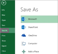
Under Save As, select a location to save your workbook. For example, click Computer to save to a folder on your desktop or computer.
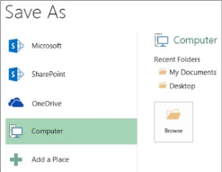
Tip: To save to your OneDrive location, click OneDrive, then sign up (or sign in). Click Add Location to add your own location to the cloud, such as Microsoft 365 SharePoint or OneDrive locations.
Click Browse to find the desired location in the Documents folder.
To choose a different location on your computer, click Desktop, then select the exact location where you want to save your workbook.
In the File name box, type a name for your new workbook. If you want to make a copy of an existing workbook, enter a different name.
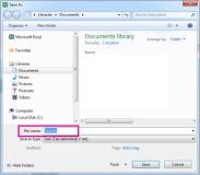
To save the workbook in a different file format (such as .xls or .txt), in the File Types list (under the File Name box), select the format you want.
Click Save.
Secure your favourite storage location
Once you have saved the workbook, you can "pin" the saved location. This makes the location available and can be used again to store another workbook. This can save you time if you tend to save many in the same folder or location. You can fix as many locations as you need.
Click File> Save As.
Under Save As, select the location where you last saved the workbook. For example, if you want to last save the workbook to your computer's Documents folder and pin the location, click Computer.
In Recent Folders on the right, point to the location you want to pin. Pushpin image the pushpin button is displayed on the right.
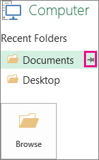
Click the image to pin the folder. The image is displayed as a pinned pushpin icon. Each time you save a workbook, this location will appear at the top of the list under Recent Folders.
Tip: To unlock the location, click the pinned pushpin image again. Fixed push pin icon.
Q42) How to edit a worksheet with the help of the Edit Worksheet Steps?
A42) Edit the worksheet to vary the design and behavior of the worksheet. For instance, you'll change the layout of worksheet data and add calculations, percentages, or totals.
To edit a worksheet with the help of the Edit Worksheet Steps

On the tabs of the Edit Worksheet dialog, you'll edit the properties of the present worksheet as follows:
See the type tab
Note: the type tab only appears for table worksheets. To sort the crosstab worksheets, select Tools> Worksheets. once you sort, the type Crosstab dialog is displayed (for more information, see the way to Sort Data during a Crosstab Worksheet).
Use the Parameters tab to manage existing parameters and make new ones (see Edit Worksheet Dialog: Parameter Tab for more information).
Click okay to save your changes and return to the worksheet.
Discoverer updates the worksheet with the changes you specify.
Note
You can also edit worksheets directly within the Discoverer workspace using drag-and-drop, right-click menus, and toolbars (see About Discoverer Plus Relational Workspaces for more information).
Q43) How to add items to a worksheet?
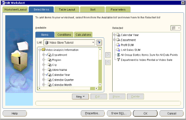
A43) If you would like to use items within the business area to research new areas of your data, add the things to your worksheet. For instance, you would possibly want to feature an item called Year to research trends over time.
For more information on creating new worksheet items (such as calculations and percentages), see the way to Create New Worksheet Items.
Tip: Click the plus (+) sign next to a folder and item to ascertain the things and values in it. Click the flashlight button above the Available box to display the Search Dialog (in Item Navigator) where you'll look for items.
Tip: To reposition worksheet items, attend the Edit Worksheet dialog: Table Layout tab or the Edit Worksheet dialog: Crosstab Layout tab and drag and drop the item. And place it on the worksheet.
Note
To quickly add a worksheet item, simply drag and drop the item from the Available Items pane into the worksheet area. To display the Available Items pane, select View> Items. Available item pane. For more information, see About dragging and dropping items within the Discoverer workspace.
To move an item from the Available list to the chosen list, do one among the following:
Q44) How to create a replacement worksheet item?
A44) Create a replacement worksheet item if you would like to research different data with items which will not be in your business area. For instance, you'll want to make a three-month mobile sales average.
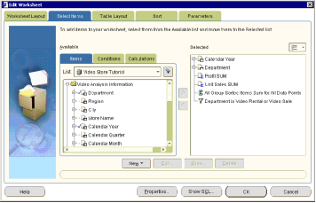
For more information on the way to add an existing item to a worksheet, see the way to Add an Item to a Worksheet.
Note
To quickly create a replacement worksheet item, select the item within the Selected Items pane and click on one among the following:
Add Item button (e.g., Add Calculation button, Add Percentage button). For more information, see About dragging and dropping items within the Discoverer workspace.
Q45) How to remove an item from a worksheet?
A45) When you not got to analyze the item, delete it from the worksheet. For instance, you'll delete a year item once you not got to analyze the info over time.
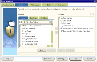
To remove an item from the worksheet:
Note
To quickly delete a worksheet item, right-click the item and select Delete. For more information, see About dragging and dropping items in the Discoverer workspace.
Q46) What are the steps of Inserting and deleting worksheets in Excel?
A46) Inserting and deleting worksheets in Excel: Steps
Q47) How do we enter data in a cell?
A47) Manually enter data into worksheet cells
If you want to enter the data manually in Excel, you have several options. You can enter data in one cell, in multiple cells at the same time, or in multiple worksheets at once. The data you enter can be numbers, text, dates, or time. You can format your data in a variety of ways. There are also some settings that you can adjust to make data entry easier.
This topic does not explain how to use data forms to enter data in worksheets. For more information on working with data forms, see Adding, Editing, Finding, and Deleting Rows Using Data Forms.
Important: If you cannot enter or edit data in a worksheet, it may be protected by you or someone else to prevent accidental changes to the data. Protected worksheets allow you to select cells to view data, but you cannot enter information in locked cells. In most cases, do not remove protection from a worksheet without the permission of the worksheet author. To unprotect a worksheet, on the Review tab, in the Changes group, click Unprotect Sheet. If a password was set when worksheet protection was applied, you must first enter that password to unprotect the worksheet.
For example, if you type 3 in the Location box and 2834 in the cell, the value is displayed as 2.834. If you type -3 in the Location box and then 283, the value is 283000.
Enter the date or time as follows:
Q48) How to Copy the formula in excel sheet?
A48)
This table summarizes how the reference type is updated if the formula containing the reference is copied two cells down and two cells to the proper.

If the reference is: | It changes to: | |
| $A$1 (absolute column and absolute row) | $A$1 |
| A$1 (relative column and absolute row) | C$1 |
| $A1 (absolute column and relative row) | $A3 |
| A1 (relative column and relative row) | C3 |
Note: Fill handle you'll also use the fill handle  to repeat a formula to an adjacent cell. After verifying that the cell reference within the formula produces the result you would like in step 4, select the cell that contains the copied formula and drag the fill handle to the world you would like to fill.
Q49) How to regroup the text in an Excel cell?
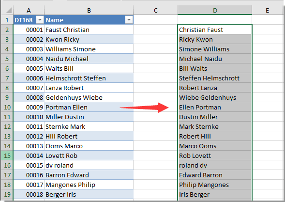
A49) Suppose you've a spreadsheet with long list names, beat the form "Last name First name", and you'd wish to relocate all the names to "First name, Last name". the thanks to achieve that? During this text, I'll show you 3 ways to help you solve your problem.
Sort text in cells using formulas
The following formulas are useful for reversing cell names and names in Excel. Please do as follows.
=TRIM (MID (b2, SEARCH (" “, b2) +1,250)) &" "&LEFT (b2, SEARCH (" “, b2)-1)

Note: within the formula, B2 is that the cell that contains the name you'd wish to relocate. Change it if necessary.
2. Still select the result cell and drag the fill handle right down to flip all the names, as shown within the screenshot below.
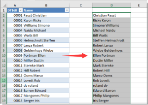
Easily rearrange the text in Excel cells.
Kutools for Excel's Text Inversion Utility allows you to easily swap text within a cell using specific Excel delimiters. See the screenshot below.
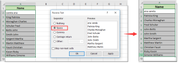
Rearrange text in cells using VBA code
In addition, you'll apply the next VBA code to invert all the names within the list directly in Excel. Please do as follows.
1. In order to open the Microsoft Visual Basic for Applications window we need to Press Alt + F11
2. within the Microsoft Visual Basic for Applications window, click Insert> Module. Then copy the next VAB code into the module window.
VBA code: Rearrange text in a cell
1 2 3 4 5 6 7 8 9 10 11 12 13 14 15 16 17
| Sub RearrangeText() 'Updated by Extendoffice 20180503 Dim xRg As Range, yRg As Range Dim LastRow As Long, i As Long Dim strTxt As String, strFs As String Dim strLs As String, N As Integer On Error Resume Next Set xRg = Application.InputBox(Prompt:="Range Selection:", _ Title:="Kutools for excel", Type:=8) For Each yRg In xRg On Error Resume Next strTxt = yRg.Value Trim (strTxt) N = InStr(strTxt, " ") strLs = Left(strTxt, N - 1) strFs = Right(strTxt, Len(strTxt) - N) yRg.Value = strFs & " " & strLs Next End Sub |
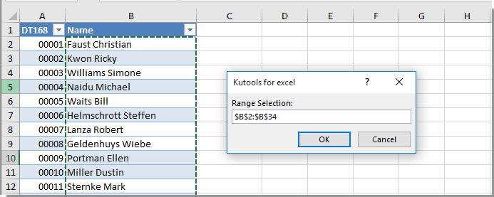
3. Next, the Kutools for Excel panel is displayed. Select the name list you'd wish to relocate and click on the OK button. See screenshot:

All "first and last names" within the chosen list are immediately flipped.
Quickly rearrange text in cells using Kutools for Excel
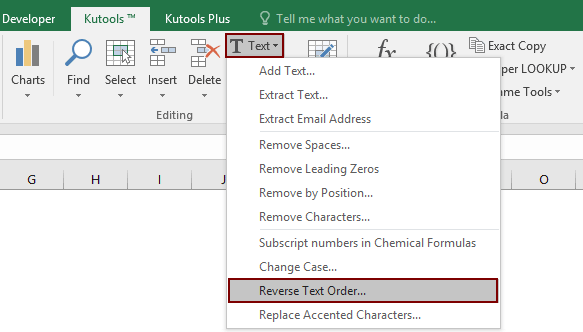
This section introduces Kutools for Excel's Reverse Text Ordering Utility to help you rearrange the text in cells.
Before using Kutools for Excel, we need to download and install it first.
2. within the Invert Text panel, select the Space option and click on on the OK button. See screenshot:
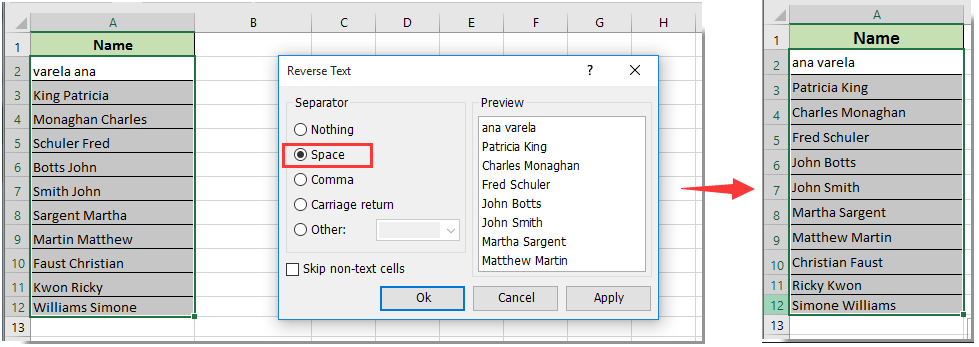
Then all the names within the chosen list are getting to be rearranged directly.
Q50) How do we create a graph between multiple worksheets / from multiple worksheets in Excel?
A50) For example, four worksheets have four tables with the same layout, as shown in the screenshot below. Next, you need to extract the data series from each worksheet to create a graph, and extract the data points from each worksheet to create a graph. How can I solve them in Excel? This article recommends two workarounds:
Extract many data series from multiple worksheets to create a graph
This section describes how to extract many data series from multiple Excel worksheets to create a column chart. You can archive by following the steps below.
2. Insert a blank chart here. Right-click on the blank graph and select Data from the right-click menu. See screenshot:
3. Open the Select Data Source dialog box and click the Add button.
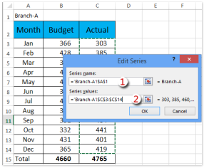
4. In the Edit Series dialog box, specify the series name and series value from the worksheet and click the OK button.
5. When you return to the Select Data Source dialog box, repeat steps 3 and 4 to add data series from other worksheets. Finally, all the data series added from the worksheet are listed in the Legend Entry (Series) box, as shown in the screenshot below.
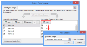
6. In the Select Data Source dialog box, click the Edit button in the Horizontal (Category) Axis Labels section to open the Axis Labels dialog box and specify the axis labels as needed. Click the [OK] button. See the screenshot above.
7. Click the OK button to close the Select Data Source dialog box
8. Optional. Continue to select the graph, click Design> Add Graph Element> Legend, and select Legend Options from the submenu. See screenshot:
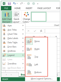
In this example, select Legend> Below.
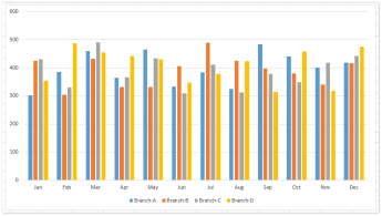
So far, you've created a clustered column chart with four data series from four worksheets. See screenshot:
Extract many data points from multiple worksheets to create a graph
You may want to create a graph whose data points are from different worksheets. This section introduces Kutools for Excel's Dynamically Browse Worksheets to extract data points from multiple worksheets into new worksheets and use these data points to create graphs.
Kutools for Excel-Includes over 300 handy tools for Excel. 30-day full-featured free trial, no credit card required! Free trial now!
1. On the Sheet tab bar, click the New button or create a new worksheet.
2. In the new worksheet, select the cell whose contents you want to extract from other worksheets and click Kutools> Other (in the Formula group)> Dynamic.
See worksheet. See screenshot:
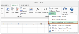
The document dynamically references Sheet 1
3. Open the Enter Worksheet Reference dialog box and do the following:
(1) Select [Fill vertically after cell] from the [Fill order] drop-down list.
(2) In the Worksheet List section, review the worksheet from which you want to extract the data points.
(3) Click the [Fill Range] button and the [Close] button in succession.
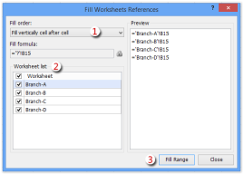
Note: If you have multiple data series with data points from different worksheets, you can repeat this step if necessary.
Then you can see that the data points are extracted from various worksheets. See screenshot:
4. Select the extracted data points and create a graph. In this example, click Insert> Insert Column Chart (or Column)> Clustered Columns to create a clustered column.
So far, you've created a clustered column chart with data points from different worksheets. See screenshot:
