Unit - 1

Introduction to linear Programming problem

Q1) Define linear programming.

A1)
This is also a really interesting topic. It starts with an easy problem, but it is often very complicated. For instance, sharing a chocolate candy between siblings may be a simple optimization problem. While solving it, we do not think mathematically. On the opposite hand, devising an e-tailer inventory and warehousing strategy are often very complex. Many SKUs with different popularity in several regions are delivered at defined times and resources.

So what's linear programming? Applied mathematics may be a simple technique that uses linear functions to represent complex relationships and find the simplest points. The important words within the preamble are drawn. The particular relationship could also be far more complicated, but it is often simplified to a linear relationship.

Linear programming applications are everywhere around you. Use applied mathematics on a private and professional side. If you're driving from home to figure and need to use the shortest route, you're using applied mathematics. Or, when delivering a project, develop a technique to figure efficiently in order that your team can deliver on time.

Q2) What are the applications of LP?

A2)

Linear programming and optimization are used in a variety of industries. Manufacturing and service industries regularly use linear programming.

1. Manufacturing uses linear programming to analyse supply chain operations.  Their motivation is to maximize efficiency with minimal operating costs. Following the recommendations of the linear programming model, manufacturers can reconfigure their storage layouts and adjust their employees to reduce bottlenecks. This is a case study of Cequent's small warehouse based in the United States. Watch this video for a clearer understanding.
2. Linear programming is also used in retail stores organized to optimize shelf space. With the number of products on the market growing exponentially, it's important to understand what your customers want. Optimization is actively used in stores such as Wal-Mart, Hyper city, Reliance, and Big Bazaar. The products in the store are strategically placed with the customer's shopping patterns in mind. The goal is to make it easier for customers to find and select the right product. This has limitations such as limited shelf space and various products.
3. Optimization is also used to optimize delivery routes. The service industry uses optimization to find the best route for multiple salespeople travelling to multiple cities. With the help of clustering and greedy algorithms, delivery routes are determined by companies such as FedEx and Amazon. The goal is to minimize operational costs and time.
4. Optimization is also used in machine learning. Supervised learning addresses the basics of linear programming. The system is trained to fit a mathematical model of a function from labelled input data that can predict values   from unknown test data.

Q3) A manufacturer produces two types of products ‘P’ and ‘Q’. Each ‘P’ type of product required 4 hours of grinding and 2 hrs of polishing, where ‘Q’ product requires 2 hrs of grinding and 5hrs of polishing.

The manufacturer has 2 grinders and 3 polishers. Each grinder works for 80hrs a week and each polisher works for 180hrs a week. Profit on ‘P’ product is Rs. 3 and profit on ‘Q’ is Rs. 4.Whatever is produced in a week is sold in the market.

How should the manufacturer allocate his capacity of production of two types of products so that he may make the maximum profit and minimum loss in a week?

A3)

Now we formulate this problem in mathematical terms as explained below-

Suppose is the number of ‘P’ product and is the number of ‘Q’ product produced weekly.

Then the weekly profit is-

Here ‘Z’ is called the objective function which is to be maximize or minimize.

Now, to produce these number of products, the total number of grinding hours needed weekly is-

And the total number of polishing hours needed per week is-

Here the number of grinding hours is not more than 80 and the number of polishing hours is not more than 180, so that we write,

This is called the first constraint]

[This is the second constraint]

Since the number of product is non-negative, then we can write-

This is called the third constraint.

Hence we form the problem mathematically as follows-

To maximize-

Subject to the constraints:

This expression is called as mathematical formulation.

Q4) Solve the following LPP graphically-

Maximize-

Subject to the constraints-

A4)

Change the given constraints into equations-

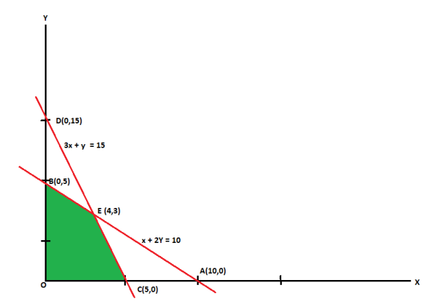
The line   meets the x-axis at the point A(10,0) and meets the y-axis at the point B(0,5). Join A and B to get the graph for the line.             

Hence origin (0,0) satisfies the inequality so that half plane containing the origin represent the solution set of .

And

The line meets the x-axis at the point C(5,0) and meets the y-axis at the point D(0,15). Join C and D to get the graph for the line.

Hence origin (0,0) satisfies the inequality   so that half plane containing the origin represent the solution set of.

Now all the points in first quadrant satisfies  .

So that first quadrant is the region represented by

Hence the region OCEBO satisfies all the inequalities.

And each point on the region is the feasible solution of the problem.

Feasible solution-

Here in this problem the feasible solution is (5,0), (4,3) and (0,5).

Now we can obtain the optimal solution of the problem.

As we know that any point in the feasible region that gives the optimal value is called an optimal solution.

The value of the objective function at corner points of the feasible region is given below-

Vertex [ feasible region ]	Value of
O(0,0)	0
C(5,0)	15
E(4,3)	18 [Maximum]
B(0,5)	10

Here we see that the maximum value of Z is 18.

Q5) Maximize

Subject to-

By using simplex method.

A5)

Here all b’s are positive and the objective function is to be maximized.

Step-1: Now express the problem in the standard form-

Let are slack variables then the problem in standard form becomes-

Maximize-

Subject to

Step-2: Find the initial basic feasible solution-

There are three equations having 5 unknowns and for obtaining the solution we assign zero value to any two of the three variables.

We start with a basic solution for which we set and .

Putting  

in the above three equations-

We get-

Here all
are positive, the basic solution is also feasible and non-degeneate.

The BFS is-

Initial BFS is given by the table below-

For

For

Similarly-

Now apply the optimality test-

As is positive under some columns, the IBFS is not optimal, we move to the next step-

Step- Identify the outgoing and incoming variables-

By the above table is the incoming variable as its incremental contribution is max. And the column in which it appears is the key column.

Dividing the  elements under b-column by the corresponding elements of key-column we find the min.positive ratio in two rows.

Therefore we arbitrarily choose the row containing as the key row.

The elements at the intersection of key row and the key column is the key element.

is therefore the outgoing variable which will now become non-basic.

Having decided that is to enter the solution we have tried to find as to what maximum under could have without violating the constraints.

So that removing , the new basis will contain as the basic variables.

Now iterate towards the optimal solution-

To transform the initial set of equations with a BFS into an equivalent set of equatins with a different BFS, we make the key element unity.

We retain the key row as it is. Then to make all other elements in key column zero, we subtract proper multiples of the key row from the other rows.

Here we subtract five times the elements of key row from the second row and three times the element of key row from the third row.

These become the second and the third of the next table.

We also change the corresponding value under column from 0 to 5.

While relacing by under the basis.

Thus the second BFS is given below-

As is either zero or negative under all columns, the above table gives the optimal BFS.

This optimal BFS is-

Q6) Maximise ‘Z’ = 2x1 + 3x2

Subject to constraints

x1 + x2 1

3x1 + x2 4

Where, x1, x2 0

A6)

Step 1: Conversion of inequalities into equalities by adding slack variables.

x1 + x2 + x3 = 1

3x1 + x2 + x4 = 4

Where x3 and x4 are slack variables.

Step 2: Identify the coefficients.

Step 3: First iteration of Simplex Method.

Therefore

Therefore, Maximum value of ‘Z’ = 3

Q7) Example)

Maximise ‘Z’ = 4x1 + 3x2

Subject to constraints

2x1 + x2 30

x1 + x2 24

Where, x1, x2 0

A7)

Step 1: Convert the inequalities into equalities adding slack variables.

2x1 + x2 + x3 = 30

x1 + x2 + x4 = 24

Where x3 and x4 are slack variables.

Step 2: Fit the data into a matrix form.

Step 3: First iteration of Simplex Method.

Therefore, Z = (0 × 30) + (0 × 24)

= 0

Step 4: Second iteration of Simplex Method.

Therefore

Step 5: Third iteration of Simplex Method.

Therefore

Z = 78

Q8) Explain two-phase method.

A8)

In the first phase of this method, the sum of the artificial variables is minimized subject to the given constraints in order to get a basic feasible solution of the LP problem. The second phase minimizes the original objective function starting with the basic feasible solution obtained at the end of the first phase.

Since the solution of the LP problem is completed in two phases, this method is called the two-phase method.

Step by step method- (Phase-I)

Step-1:

(a)  If all the constraints in the given LP problem are ‘less than or equal to’ (≤) type, then Phase II can be directly used to solve the problem. Otherwise, the necessary number of surplus and artificial variables are added to convert constraints into equality constraints.

(b) If the given LP problem is of minimization, then convert it to the maximization type by the usual method.

Step-2: Assign zero coefficient to each of the decision variables (xj) and to the surplus variables; and assign – 1 coefficient to each of the artificial variables. This yields the following auxiliary LP problem.

Subject to the constraints

And

Step 3: Apply the simplex algorithm to solve this auxiliary LP problem. The following three cases may arise

At optimality.

(a) Max Z * = 0 and at least one artificial variable is present in the basis with positive value. This means that no feasible solution exists for the original LP problem.

(b) Max Z * = 0 and no artificial variable is present in the basis. This means that only decision variables

(xj’s) are present in the basis and hence proceed to Phase II to obtain an optimal basic feasible solution on the original LP problem.

(c) Max Z * = 0 and at least one artificial variable is present in the basis at zero value. This means that a feasible solution to the auxiliary LP problem is also a feasible solution to the original LP problem. In order to arrive at the basic feasible solution, proceed directly to Phase II or else eliminate the artificial basic variable and then proceed to second phase.

Second phase- Assign actual coefficients to the variables in the objective function and zero coefficient to the artificial variables which appear at zero value in the basis at the end of Phase I. The last simplex table of Phase I can be used as the initial simplex table for Phase II. Then apply the usual simplex algorithm to the modified simplex table in order to get the optimal solution to the original problem. Artificial variables that do not appear in the basis may be removed.

Q9) By using two phase method solve the following LPP,

Subject to the constraints,

And

A9)

Convert the function into maximization form and add surplus variables and artificial variables and in the constraints, it becomes,

Subject to the constraints

And

Where,

First phase-

This phase starts by considering the following auxiliary LP problem:

Subject to the constraints

The initial solution is given in table,

Artificial variables and are now removed, one after the other, maintaining the feasibility of the solution.

First iteration- Applying the following row operations to get an improved solution by entering variable in the basis and first removing variable from the basis. The improved solution is shown in next table

Note-the variable cannot be entered into the basis as this would lead to an infeasible solution.

*- we can permanently remove this column at this stage

Second iteration: To remove from the solution shown in above, we enter variable s2 in the basis by applying the following row operations. The new solution is shown in next table. It may be noted that if instead of , variable is chosen to be entered into the basis, it will lead to an infeasible solution

* Remove columns and from table

Since all  – 0 correspond to non-basic variables, the optimal solution: = 0, = 4,

= 0, = 21, = 0, = 0 with Z* = 0 is arrived at. However, this solution may or may not be the basic feasible solution to the original LP problem. Thus, we have to move to Phase 2 to get an optimal solution to our original LP problem.

Second phase-

The modified simplex table obtained from Table given above is

First iteration:

Introducing variable into the basis and removing variable from the basis by applying the following row operations:

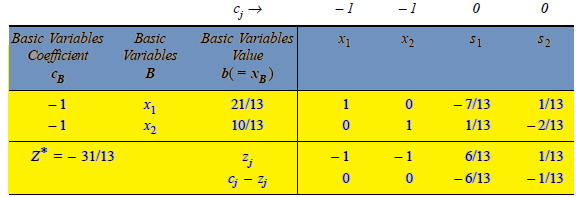
The improved basic feasible solution so obtained is given in next table. Since in next table,  – for all non-basic variables, the current solution is optimal. Thus, the optimal basic feasible solution to the given

LP problem is:   = 21/13, = 10/13 and Max = – 31/13 or Min Z = 31/13.

Q10) Solve the following LPP by using Big-M method)

Subject to the constraints,

And

A10)

Here all constraints of the given LPP are equations, therefore only artificial variables and are added in the constraints to convert given LP problem to its standard form. The standard form of the problem is stated as follows:

Subject to the constraints,

And

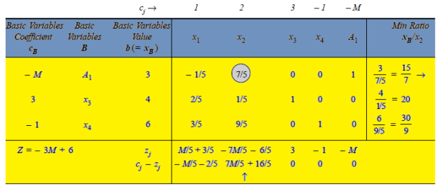
An initial basic feasible solution is-

Since value of –   in Table given above is the largest positive value, the non-basic variable x3 is chosen to replace the artificial variable A2 in the basis. Thus, to get an improved solution, apply the following row operations.

The improved basic feasible solution will be

Since value of – > 0 (positive) in Table above, the non-basic variable x2 is chosen to replace the artificial variable A1 in the basis. Thus, to get an improved basic feasible solution, apply the following row operations:

The improved basic feasible solution will be

Once again, the solution shown in Table above is not optimal as – > 0  in -column. Thus, applying the following row operations for replacing non-basic variable in the basis with basic variable x4:

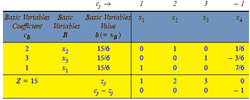
The improved basic feasible solution will be,

Since all – , therefore, we get an optimal solution with value of variables as: = 15/6, = 15/6, = 15/6 and Max Z = 15.

Q11) What are the steps for big-M method?

A11)

1. Express the problem in the standard form by using slack, surplus and artificial variables.

2. Select slack variables and artificial variables as the initial basic variables with the cost coefficients as '0' or '-M' respectively.

3. Use simplex procedure for iterations & obtain optimum solution. During the iterations, one can notice that the artificial variables leave the basis first and then the slack variables with improved value of objective function at each iteration to obtain the optimum solution.

Q12) What is infeasibility?

A12)

Infeasibility is a condition that arises when constraints are inconsistent (mutually exclusive) i.e. no value of the variables satisfy all the constraint simultaneously. This results in infeasible solution. If two or more constraints of a linear programming problem are mutually conflicting, it does not have a feasible solution.