undefined | unit 3 the greedy method

Back to Study material

DAA

Unit 3The Greedy Method Q1) Describe job sequencing with deadline?A1) Job Sequencing with Deadlines

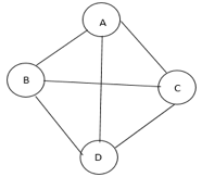
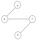
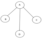
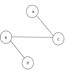
As below, the problem is mentioned.

● N jobs are to be stored on a computer.

● Each job has a di-0 deadline and a pi-0 benefit.

● Pi is won when the job is done by the deadline.

● If it is processed for unit time on a computer, the job is done.

● There is only one computer available to process work.

● Just one job on the computer is processed at a time.

● A effective approach is a subset of J jobs such that each job is done by its deadline.

A feasible solution with optimum benefit potential is an optimal solution.

Example : Let n = 4, (p1,p2,p3,p4) = (100,10,15,27), (d1,d2,d3,d4) = (2,1,2,1)

No. feasible solution processing sequence profit value

i (1,2) (2,1) 110

ii (1,3) (1,3) or (3,1) 115

iii (1,4) (4,1) 127

iv (2,3) (2,3) 25

v (3,4) (4,3) 42

vi (1) (1) 100

vii (2) (2) 10

viii (3) (3) 15

ix (4) (4) 27

● Consider the workers subject to the constraint that the resulting work sequence J is a feasible solution in the non-increasing order of earnings.

● The non-increasing benefit vector is in the example considered before,

(100 27 15 10) (2 1 2 1)

p1 p4 p3 p2 d1 d d3 d2

J = { 1} is a feasible one

J = { 1, 4} is a feasible one with processing sequence ( 4,1)

J = { 1, 3, 4} is not feasible

J = { 1, 2, 4} is not feasible

J = { 1, 4} is optimal

Theorem:

Let J be a set of K jobs and

Σ = (i1,i2,….ik) be a permutation of jobs in J such that di1 ≤ di2 ≤…≤ dik.

● J is a feasible solution that can be processed in order without breaching any deadly jobs in J.

Proof :

● If the jobs in J can be processed in order without violating any deadline by specifying the feasible solution, then J is a feasible solution.

● Therefore, we only have to show that if J is a feasible one, then ⁇ is a possible order in which the jobs can be processed.

● Suppose J is a feasible solution. Then there exists Σ1 = (r1,r2,…,rk) such that

drj ≥ j, 1 ≤ j <k

i.e. dr1 ≥1, dr2 ≥ 2, …, drk ≥ k.

each job requiring an unit time

Σ= (i1,i2,…,ik) and Σ 1 = (r1,r2,…,rk)

Assume Σ 1 ≠ Σ. Then let a be the least index in which Σ 1 and Σ differ. i.e. a is such that ra ≠ ia.

Let rb = ia, so b > a (because for all indices j less than a rj = ij).

In Σ 1 interchange ra and rb. • Σ = (i1,i2,… ia ib ik ) [rb occurs before ra

in i1,i2,…,ik] • Σ 1 = (r1,r2,… ra rb … rk )

i1=r1, i2=r2,…ia-1= ra-1, ia ≠ rb but ia = rb

We know di1 ≤ di2 ≤ … dia ≤ dib ≤… ≤ dik.

Since ia = rb, drb ≤ dra or dra ≥ drb.

In the feasible solution dra ≥ a drb ≥ b

● Therefore, if ra and rb are exchanged, the resulting permutation Σ11 = (s1, ... sk) reflects an order with the least index in which Σ11 and Σ differ by one is increased.

● The jobs in Σ 11 can also be processed without breaking a time limit.

● Continuing in this manner, ⁇ 1 can be translated into ⁇ without breaching any time limit.

● The theorem is thus proven.

Q2) Explain a general method?A2) General methodsA greedy algorithm is any algorithm that follows the problem solving metaheuristic of making the locally optimal choice at each stage with the hope of finding the global optimum.General Method:Often we are looking at optimization problems whose performance is exponential.• For an optimization problem, we are given a set of constraints and an optimization function.● Solutions that satisfy the constraints are called feasible solutions.● A feasible solution for which the optimization function has the best possible value is called an optimal solution.● Cheapest lunch possible: Works by getting the cheapest meat, fruit, vegetable, etc.● By a greedy method we attempt to construct an optimal solution in stages.● At each stage we make a decision that appears to be the best (under some criterion) at the time.● A decision made at one stage is not changed in a later stage, so each decision should assure feasibility.Greedy algorithms produce good solutions on some mathematical problems, but not on others. Most problems for which they work well have two properties:Greedy choice property We can make whatever choice seems best at the moment and then solve the sub problems that arise later. The choice made by a greedy algorithm may depend on choices made so far but not on future choices or all the solutions to the sub problem. It iteratively makes one greedy choice after another, reducing each given problem into a smaller one. In other words, a greedy algorithm never reconsiders its choices. This is the main difference from dynamic programming, which is exhaustive and is guaranteed to find the solution. After every stage, dynamic programming makes decisions based on all the decisions made in the previous stage, and may reconsider the previous stage's algorithmic path to solution. Optimal substructure "A problem exhibits optimal substructure if an optimal solution to the problem contains optimal solutions to the sub-problems."Greedy method suggests that one can devise an algorithm that works in stages, considering one input at a time. At each stage, a decision is made regarding whether a particular input is an optimal solution. This is done by considering the inputs in an order determined by some selection procedure.

Algorithm Greedy (a, n)

//a [1: n] contains the n inputs.

{

solution:= ø; //Initialize the solution.

for i:=1 to n do

{

x:= Select(a);

if Feasible(solution, x) then

solution: = Union(Solution, x);

}

return solution;

}

The function Select selects an input from a[ ] and removes it. The selected input value is assigned to x. Feasible is a Boolean valued function that determines whether x can be included into the solution vector. Union combines x with the solution and updates the objective function.Consider change making: ● Given a coin system and an amount to make change for, we want minimal number of coins.● A greedy criterion could be, at each stage increase the total amount of change constructed as much as possible.● In other words, always pick the coin with the greatest value at every step.● A greedy solution is optimal for some change systems.Machine scheduling:● Have a number of jobs to be done on a minimum number of machines. Each job has a start and end time. Order jobs by start time.● If an old machine becomes available by the start time of the task to be assigned, assign the task to this machine; if not assign it to a new machine.● This is an optimal solution.● Note that our Huffman tree algorithm is an example of a greedy algorithm:● Pick least weight trees to combine. Q3) What do you mean by knapsack problem?A3) Knapsack Problem Problem description:● Pack a knapsack with a capacity of c.● From a list of n items, we must select the items that are to be packed in the knapsack.● Each object i has a weight of i w and a profit of i p .● In a feasible knapsack packing, the sum of the weights packed does not exceed the knapsack capacity. ● Let xi = 1 when item i is selected and let xi = 0 when item i is not selected.Maximize

Subject to

And 0<=xi<=1, 1<=i<=nAll profits and weights are positiveWe are to find the values of i x where =1 i x if object i is packed into the knapsack and = 0 i x if object i is not packed.Greedy strategies for this problem:● From the remaining objects, select the object with maximum profit that fits into the knapsack.● From the remaining objects, select the one that has minimum weight and also fits into the knapsack.● From the remaining objects, select the one with maximum i i p / w that fits into the knapsack.We can also state the knapsack problem in the following way.Input: A weight capacity C, and n items of weights W[1:n] and monetary value P[1:n]. Problem: Determine which items to take and how much of each item so that ● the total weight is <= C, and ● the total value (profit) is maximized. Formulation of the problem:

Let x[i] be the fraction taken from item i. 0 <= x[i] <= 1.

The weight of the part taken from item i is x[i]*W[i]

The Corresponding profit is x[i]*P[i]

The problem is then to find the values of the array x[1:n] so that x[1]P[1]+x[2]P[2]+...+x[n]P[n] is maximized subject to the constraint that x[1]W[1]+x[2]W[2]+...+x[n]W[n] <= C

Greedy selection policy: three natural possibilities

Policy 1: Choose the lightest remaining item, and take as much of it as can fit.
Policy 2: Choose the most profitable remaining item, and take as much of it as can fit.
Policy 3: Choose the item with the highest price per unit weight (P[i]/W[i]), and take as much of it as can fit.

Policy 3 always gives an optimal solution.

Q4) Define minimum spanning tree?A4) Minimum Spanning TreeIn the Greedy approach MST (Minimum Spanning Trees) is used to find the cost or the minimum path. Let G= (V, E) be an undirected connected graph, also T= (V’, E’) be a subgraph of the spanning tree G if and only if T is a tree. Spanning trees are usually used to get an independent set of circuit’s equations in the electrical network. Once the spanning tree is obtained, suppose B is a set of edges not present in the spanning tree then adding one edge from B will form an electrical cycle. A spanning tree is a minimal subgraph G’ of G such that V (G’) =V (G) and G’ is connected by minimal subgraph. Any connected graph with n vertices must have at least n-1 edges and all connected graphs with n-1 edges are trees. The spanning trees of G will represent all feasible choices. The best spanning tree is tree with minimum cost. The cost of the spanning tree is nothing but the sum of the cost of the edges in that tree. Any tree consisting of edges of a graph and including all the vertices of the graph is known as a “Spanning Tree”.

Fig : graph with verticesThe above figure shows a graph with four vertices and some of its spanning tree are shown as below:

Fig : spanning treeQ5) Write the pillars of greedy algorithm?A5) In general, greedy algorithms have five pillars:

A candidate set, from which a solution is created

A selection function, which chooses the best candidate to be added to the solution

A feasibility function, that is used to determine if a candidate can be used to contribute to a solution

An objective function, which assigns a value to a solution, or a partial solution, and

A solution function, which will indicate when we have discovered a complete solution

Q6) Write the algorithm for job sequencing with deadline?A6) Algorithm for job Sequencing with Deadline

GREEDY ALGORITHM FOR JOB SEQUENCING WITH DEADLINE

Procedure greedy job (D, J, n) J may be represented by

// J is the set of n jobs to be completed // one dimensional array J (1: K)

// by their deadlines // The deadlines are

J ← {1} D (J(1)) ≤ D(J(2)) ≤ .. ≤ D(J(K))

for I 2 to n do To test if JU {i} is feasible,

If all jobs in JU{i} can be completed we insert i into J and verify

by their deadlines D(J®) ≤ r 1 ≤ r ≤ k+1 then J

J← U{I}

end if

repeat

end greedy-job

Procedure JS(D,J,n,k)

// D(i) ≥ 1, 1≤ i ≤ n are the deadlines //

// the jobs are ordered such that //

// p1 ≥ p2 ≥ ……. ≥ pn //

// in the optimal solution ,D(J(i) ≥ D(J(i+1)) //

// 1 ≤ i ≤ k //

integer D(o:n), J(o:n), i, k, n, r

D(0)← J(0) ← 0

// J(0) is a fictitious job with D(0) = 0 //

K←1; J(1) ←1 // job one is inserted into J //

for i ← 2 to do // consider jobs in non increasing order of pi //

// find the position of i and check feasibility of insertion //

r ← k // r and k are indices for existing job in J //

// find r such that i can be inserted after r //

while D(J(r)) > D(i) and D(i) ≠ r do

// job r can be processed after i and //

// deadline of job r is not exactly r //

r ← r-1 // consider whether job r-1 can be processed after i //

repeat

if D(J(r)) ≥ d(i) and D(i) > r then

// the new job i can come after existing job r; insert i into J at position r+1 //

for I ← k to r+1 by –1 do

J(I+1) J(l) // shift jobs( r+1) to k right by//

//one position //

repeat

if D(J(r)) ≥ d(i) and D(i) > r then

// the new job i can come after existing job r; insert i into J at position r+1 //

for I k to r+1 by –1 do

J(I+1) ← J(l) // shift jobs( r+1) to k right by//

//one position //

Repeat

Complexity analysis :

● Let the number of jobs be n and the number of jobs used in the solution be s.

● The loop is iterated (n-1)times between lines 4-15 (the for-loop).

● Each iteration requires O(k) where k is the number of jobs that exist.

● The algorithm requires 0(sn) s ≤ n time, so 0(n2 ) is the worst case time.

If di = n - i+1 1 ≤ i ≤ n, JS takes θ(n2 ) time

D and J need θ(s) amount of space.

Q7) Write any example of a knapsack problem?A7) Example

i: 1 2 3 4

P: 5 9 4 8

W: 1 3 2 2

C= 4

P/W: 5 3 2 4

Solution:

1st: all of item 1, x[1]=1, x[1]*W[1]=1

2nd: all of item 4, x[4]=1, x[4]*W[4]=2

3rd: 1/3 of item 2, x[2]=1/3, x[2]*W[2]=1

Now the total weight is 4=C

(x[3]=0)

Algorithm GreedyKnapsack (m, n)

//p[1:m] and w[1:n] contain the profits and weights respectively of the n objects ordered //such that p[i]/w[i]>= p[i+1]/w[i+1]. m is the knapsack size and x[1:n] is the solution vector.

{

for i:=1 to n do x[i]:= 0.0; //initialize x.

U:= m;

for i:=1 to n do

{

if(w[i]>U) then break;

x[i]:=1.0;

U:=U-w[i];

}

if(i<=n) then x[i]:= U/w[i];

}

Q8) Write the prim’s algorithm?A8) Prim’s Algorithm ● If A is the set of edges selected so far, then A forms a tree.● The next edges (u,v) to be included in A is a minimum cost edge not in A with the property that A U {u, v} is also a tree.● Steps to solve the prim's algorithm:Step 1: remove all loops and parallel edgesStep 2: chose any arbitrary node as root nodeStep 3: check the outgoing edges and chose edge with the less valueStep 4: find the optimal solution by adding all the minimum cost of edges.Algorithm Prim(E, cost, n, t)

//E is the set of edges in G cost (1:n,1:n) is the adjacency matrix such at cost (i,j) is a +ve //real number or cost (i,j) is ∞ if no edge (i,j) exists. A minimum cost spanning tree is //computed and stored as a set of edges in the array T (1:n-1,1:2). (T(i,1), T(i,2) is an edge //in minimum cost spanning tree. The final cost is returned.

{

Let (k,l) to be an edge of minimum cost in E;

mincost ß cost (k,l);

(T(1,1) T(1,2) )ß (k,l);

for iß 1 to n do // initialing near

if cost (i,L) < cost (I,k) then near (i) ß L ;

else near (i) ß k ;

near(k) ß near (l) ß 0;

for i ß 2 to n-1 do

{

//find n-2 additional edges for T

Let j be an index such that near (J) ¹ 0 and

cost (J, near(J)) is minimum;

(T(i,1),T(i,2)) ß (j, NEAR (j));

mincost ß mincost + cost (j, near (j));

near (j) ß 0;

for k ß 1 to n do // update near[]

if near (k) ¹ 0 and cost(k near (k)) > cost(k,j) then NEAR (k) ß j;

}

return mincost;

}

Q9) Explain kruskal's algorithm?A9) Kruskal’s Algorithm Kruskal's algorithm is an algorithm in graph theory that finds a minimum spanning tree for a connected weighted graph. This means it finds a subset of the edges that forms a tree that includes every vertex, where the total weight of all the edges in the tree is minimized. If the graph is not connected, then it finds a minimum spanning forest (a minimum spanning tree for each connected component). Kruskal's algorithm is an example of a greedy algorithm.In Kruskal’s algorithm● The edges are considered in the non-decreasing order.● To get the minimum cost spanning tree, the set of edges so far considered may not be a tree.● T will be a forest since the set of edges T can be completed into a tree iff there are no cycles in T. Implementation issues in Kruskal’s algorithm for minimum cost spanning tree● A tree with (n) vertices has (n: 1) edges ● Minheap is used to delete minimum cost edge. ● To make sure that the added edge (v, w) does not form a cycle in T, (to add to T), we use UNION and Find algorithms of sets.● The vertices are grouped in such a way that all the vertices in a connected component are placed into a set. Two vertices are connected in T iff they are in the same set. Algorithm Kruskal (E, cost, n, t)

//E is the set of edges in G. G has n vertices cost (u, v) is the cost of edge (u , v) t is //the set of edges in the minimum cost spanning tree and mincost is the cost. The //final cost is returned.

{

Construct the heap out of the edges cost using Heapify;

for i:=1 to n do Parentß-1 //Each vertex is in the different set

iß mincostß 0;

While (i < n -1) and (heap not empty) do

{

delete a minimum cost edge (u,v) from the heap and reheapify using ADJUST;

JßFIND (u); kßFIND (v);

If j ≠ k then ißi+1

{ T(i, 1) ß u; T (i,2) ßv;

Mincost ß mincost + cost(u,v);

union (j, k);

}

if (i ≠ n-1) then write(“no spanning tree”);

else return minsort;

}

Complexities:

● The edges are maintained as a min heap.

● The next edge can be obtained / deleted in O(log e) time if G has e edges.

● Reconstruction of heap using ADJUST takes O(e) time.

Kruskal’s algorithm takes O(e loge) time .

Efficiency :

Kruskal's algorithm's efficiency is dependent on the time taken to sort the edge weights of a given graph.

● With an effective algorithm for sorting: Efficiency: Θ(|E| log |E|)

Q10) Explain dijkstra algorithm?A10) Dijkstra AlgorithmStrategy: from the set of "unfinished" nodes, pick up the node v whose path-weight (from the source) is shortest in the set, mark this node v to be “finished” (shortest path is now found for this node), and update the path-weights to the other unfinished nodes adjacent to the just-finished node v, using the direct edges from this node v.Initialization: Each node not having an edge with the source node is initialized with distance (shortest from the source) = infinity, and the source is marked as finished.Input: Weighted graph, a “source” node s [can not handle neg cycle]Output: Shortest distance to all nodes from the source sAlgorithm Dijkstra

Step 1. s.distance = 0; // shortest distance from s

Step 2. mark s as “finished”; //shortest distance to s from s found

Step 3. For each node w do

Step 4. if (s, w) ϵ E then w.distance= Dsw else w.distance = inf;

// O(N)

Step 5. While there exists a node not marked as finished do

// Θ(|N|), each node is picked once & only once

Step 6. v = node from unfinished list with

the smallest v.distance;

// loop on unfinished nodes O(N): total O(N2)

Step 7. mark v as “finished”; // why?

Step 8. For each edge (v, w) ϵ E do //adjacent to v: Θ(|E|)

Step 9. if (w is not “finished” &

(v. distance + Dvw < w.distance) ) then

Step 10. w.distance = v.distance + Dvw;

// Dvw is the edge-weight from

// current node v to w

Step 11. w.previous = v;

// v is parent of w on the shortest path

end if;

end for;

end while;

End algorithm

Complexity:

(1) The while loop runs N-1 times: [Θ(N)], find-minimum-distance-node v runs another Θ(N) within it, thus the complexity is Θ(N2);

Can you reduce this complexity by a Queue?

(2) for-loop, as usual for adjacency list graph data structure, runs for |E| times including the outside while loop.

Grand total: Θ(|E| + N2) = Θ(N2), as |E| is always ≤ N2.

To store the priority queue, use an unordered array: Efficiency = x (n2).

Store the priority queue using min-heap: Performance = O (m log n)

Sign Up