undefined | unit 5 decrease and conquer approaches space time tradeoffs

DAA

Unit 5Decrease and Conquer Approaches, Space-Time Tradeoffs Q1) What is decrease and conquer approaches?A1) Decrease and Conquer Approaches Decrease & conquer is a general strategy of algorithm design focused on the manipulation of the relationship between a solution to a given problem instance and a solution to a smaller example of the same problem. Top-down (recursive) or bottom-up (non-recursive) manipulation may be used. Implementation:This technique can be applied either top-down or bottom-up.Top - down approach: It often contributes to the recursive execution of the problem.Bottom - up approach: It is generally applied in an iterative fashion, beginning with a solution to the smallest example of the problem. Variations: The key variants of decrease and conquest are

Decrease by a constant: In this variation, the size of an instance in each iteration of the algorithm is decreased by the same constant. Usually, this constant is equal to one, although other constant size reductions do happen occasionally.

Example issues are given below:a. insertion sort b. graph traversal algorithms (DFS and BFS) c. topological sorting d. algorithms for generating permutations, subsets

Fig: Decrease by a constant (usually by 1)

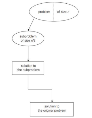
2. Decrease by a constant factor: On each iteration of the algorithm, this technique suggests decreasing a problem instance by the same constant factor. This constant factor is equivalent to two in most applications. A decrease by a factor other than two is extremely uncommon.

Algorithms that decrease by a constant factor are very effective, especially when the factor is greater than 2 as in the fake-coin problem. Example issues are given below:a. binary search and bisection method

Fig: Decrease by a constant factor (usually by half)

3. Variable size decrease: The size-reduction pattern in this variation differs from one iteration of an algorithm to another.

As the value of the second statement is always smaller on the right-hand side than on the left-hand side in the problem of finding gcd of two numbers, it does not decrease by either a constant or a constant element. Example issues are given below:a. Euclid ‘s algorithm Q2) Describe insertion sort?A2) Insertion Sort Insertion style is a decrease & conquer technique application. It is a sort based on comparison in which the sorted array is constructed on one entry at a time.Insertion sorting is a very basic process for sorting numbers in an ascending or descending order. The gradual method is accompanied by this method. It can be contrasted with the method of sorting cards at the time of playing a game.The numbers that are needed to be sorted are known as keys. Here is the insertion sort method algorithm. Algorithm:

Algorithm: Insertion-Sort (A)

for j = 2 to A.length

key = A[j]

// Insert A[j] into the sorted sequence A[1.. j - 1]

i = j - 1

while i > 0 and A[i] > key

A[i + 1] = A[i]

i = i -1

A[i + 1] = key

Analysis:This algorithm's run time is very dependent on the input given. If the numbers given are sorted, this algorithm runs in O(n) time. If the numbers given are in reverse order, the algorithm runs in O(n2) time. Example:

Using insertion sort to sort the following list of elements:

89, 45, 68, 90, 29, 34, 17

89 |45 68 90 29 34 17

45 89 |68 90 29 34 17

45 68 89 |90 29 34 17

45 68 89 90 |29 34 17

29 45 68 89 90 |34 17

29 34 45 68 89 90 |17

17 29 34 45 68 89 90

Application:In the following instances, the insertion sort algorithm is used:● When only a few elements are in the list.● When there are few elements for sorting. Advantages:

Straightforward implementation. Three variants exist.

Left to right scan

Right to left scan

Binary insertion sort

2. Effective on a small list of components, on a nearly sorted list.3. In the best example, running time is linear.4. This algorithm is stable.5. Is the on-the-spot algorithm Q3) Write the difference between DFS and BFS?A3) Difference between DFS and BFS

BFS	DFS
BFS, stands for Breadth First Scan.	DFS, which stands for First Search Depth
For finding the shortest path, BFS uses Queue.	For finding the shortest path, DFS uses Stack.
It is not ideal for the decision tree used in puzzle games, as BFS considers all neighbours.	DFS is best suited to the decision tree. As with one decision, in order to raise the decision, we need to go further. If we come to a decision, we'll win.
When the target is nearer to the source, the BFS is higher.	When the goal is far from the source, the DFS is better
Time BFS Complexity = O(V+E) where vertices are V and edges are E.	DFS Time Complexity is also O(V+E) where vertices are V, and edges are E.
BFS has been slower than DFS.	DFS is quicker than BFS.

Q4) Explain depth first search?A4) Depth First Search (DFS)Depth First Search is an algorithm for traversing or searching a graph.It starts from some node as the root node and the explores each and every branch of that node before backtracking to the parent node.DFS is an uninformed search that progresses by expanding the first child node of the graph that appears and thus going deeper and deeper until a goal node is found, or until it hits a node that has no children.Then the search backtracks, returning to the most recent node it hadn't finished exploring. In a non-recursive implementation, all freshly expanded nodes are added to a LIFO stack for expansion.Steps for implementing Depth first search Step 1: - Define an array A or Vertex that store Boolean values, its size should be greater or equal to the number of vertices in the graph G.Step 2: - Initialize the array A to false Step 3: - For all vertices v in G if A[v] = false process (v)Step 4: - Exit Algorithm for DFS

DFS(G)

{

for each v in V, //for loop V+1 times

{

color[v]=white; // V times

p[v]=NULL; // V times

}

time=0; // constant time O(1)

for each u in V, //for loop V+1 times

if (color[u]==white) // V times

DFSVISIT(u) // call to DFSVISIT(v) , at most V times O(V)

}

DFSVISIT(u)

{

color[u]=gray; // constant time

t[u] = ++time;

for each v in Adj(u) // for loop

if (color[v] == white)

{

p[v] = u;

DFSVISIT(v); // call to DFSVISIT(v)

}

color[u] = black; // constant time

f[u]=++time; // constant time

}

DFS algorithm used to solve following problems: ● Testing whether graph is connected.● Computing a spanning forest of graph.● Computing a path between two vertices of graph or equivalently reporting that no such path exists.● Computing a cycle in graph or equivalently reporting that no such cycle exists. Analysis of DFSIn the above algorithm, there is only one DFSVISIT(u) call for each vertex u in the vertex set V. Initialization complexity in DFS(G) for loop is O(V). In second for loop of DFS(G) , complexity is O(V) if we leave the call of DFSVISIT(u).Now, Let us find the complexity of function DFSVISIT(u)The complexity of for loop will be O(deg(u)+1) if we do not consider the recursive call to DFSVISIT(v). For recursive call to DFSVISIT(v), (complexity will be O(E) as Recursive call to DFSVISIT(v) will be at most the sum of degree of adjacency for all vertex v in the vertex set V. It can be written as ∑ |Adj(v)|=O(E) vεVThe running time of DSF is (V + E). Q5) Describe breadth first search?A5) Breadth First Search It is an uninformed search methodology which first expand and examine all nodes of graph systematically in search of the solution in the sequence and then go at the deeper level. In other words, it exhaustively searches the entire graph without considering the goal until it finds it.From the standpoint of the algorithm, all child nodes obtained by expanding a node are added to a FIFO queue. In typical implementations, nodes that have not yet been examined for their neighbors are placed in some container (such as a queue or linked list) called "open" and then once examined are placed in the container "closed". Steps for implementing Breadth first search

Step 1: - Initialize all the vertices by setting Flag = 1

Step 2: - Put the starting vertex A in Q and change its status to the waiting state by setting Flag = 0

Step 3: - Repeat through step 5 while Q is not NULL

Step 4 : - Remove the front vertex v of Q . process v and set the status of v to the processed status by setting Flag = -1

Step 5: - Add to the rear of Q all the neighbour of v that are in the ready state by setting Flag = 1 and change their status to the waiting state by setting flag = 0

Step 6: - Exit

Algorithm for BFS

BFS(G,s)

{

for each v in V - {s} // for loop {

color[v]=white;

d[v]= INFINITY;

p[v]=NULL;

}

color[s] = gray;

d[s]=0;

p[s]=NULL;

Q = ø; // Initialize queue is empty

Enqueue(Q,s); /* Insert start vertex s in Queue Q */

while Q is nonempty // while loop

{

u = Dequeue[Q]; /* Remove an element from Queue Q*/

for each v in Adj[u] // for loop

{ if (color[v] == white) /*if v is unvisted*/

{

color[v] = gray; /* v is visted */

d[v] = d[u] + 1; /*Set distance of v to no. of edges from s to u*/

p[v] = u; /*Set parent of v*/

Enqueue(Q,v); /*Insert v in Queue Q*/

}

color[u] = black; /*finally visted or explored vertex u*/

}

Breadth First Search algorithm used in ● Prim's MST algorithm. ● Dijkstra's single source shortest path algorithm. ● Testing whether graph is connected.● Computing a cycle in graph or reporting that no such cycle exists.Analysis of BFSIn this algorithm first for loop executes at most O(V) times.While loop executes at most O(V) times as every vertex v in V is enqueued only once in the Queue Q. Every vertex is enqueued once and dequeued once so queuing will take at most O(V) time. Inside while loop, there is for loop which will execute at most O(E) times as it will be at most the sum of degree of adjacency for all vertex v in the vertex set V.Which can be written as

∑ |Adj(v)|=O(E)

vεVTotal running time of BFS is O(V + E).Like depth first search, BFS traverse a connected component of a given graph and defines a spanning tree.Space complexity of DFS is much lower than BFS (breadth-first search). It also lends itself much better to heuristic methods of choosing a likely-looking branch. Time complexity of both algorithms are proportional to the number of vertices plus the number of edges in the graphs they traverse. Q6) Define DFS method of topological sorting with example?A6) Topological sorting is a sorting method for listing the graph's vertices in such an order that the vertex where the edge begins is classified before the vertex where the edge ends for each edge in the graph.It is possible to solve the topological sorting problem by using1. DFS method 2. Source removal methodDFS Method (Order Popped)● Output the topological sorting, reverse the orderExample To solve the topological sorting issue for the given graph, apply the DFS-based algorithm:

Step	graph	Remark
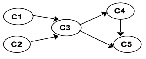
1		Insert C1 into stack. C1 (1)
2		Insert C2 into stack. C2 (2) C1 (1)
3		Insert C4 into stack C4 (3) C2 (2) C1(1)
4		Insert C5 into stack C5 (4) C4 (3) C2 (2) C1(1)
5	NO adjacent vertex for C5, backtrack, unvisited	Delete C5 from stack C5 (4, 1) C4 (3) C2 (2) C1(1)
6	NO adjacent vertex for C4, backtrack, unvisited	Delete C4 from stack C5 (4, 1) C4 (3, 2) C2 (2) C1(1)
7	NO adjacent vertex for C3, backtrack, unvisited	Delete C3 from stack C5 (4, 1) C4 (3,2) C2 (2, 3) C1(1)
8	NO adjacent vertex for C1, backtrack, unvisited	Delete C1 from stack C5 (4, 1) C4 (3,2) C2 (2, 3) C1(1, 4)
The stack is empty, but there is an unvisited node, so start the DFS again by arbitrarily selecting an unvisited node as the source.
9		Insert C2 into stack C5 (4, 1) C4 (3,2) C2 (2, 3) C1(1, 4) C2(5)
10	NO adjacent vertex for C2, backtrack, unvisited	Delete C2 from stack C5 (4, 1) C4 (3,2) C2 (2, 3) C1(1, 4) C2(5, 5)
The stack is empty, leaving NO unvisited node, so the algorithm stops. Off order the popping-off order is: C5, C4, C3, C1, C2, List sorted topologically (reverse of pop order): C2, C1 C3 C4 C5

Q7) Explain source removal method?A7) Source Removal Method ● Centered solely on decrease & conquer.● Identify a source repeatedly in the remaining digraph, which is a vertex with no Edges inbound.● Remove it and all of the edges that come out of it. Example:Apply the algorithm based on Source Removal to solve the topological sorting problem for the given graph:

Solution:

The topological order is C1, C2, C3, C4, C5 Q8) What is sorting by counting?A8) Sorting by Counting Suppose the elements to be sorted belong, with possible repetition, to a known set of small values between l and u.Constraint: the original Distribution Counting list can not be overwritten: measure the frequency of each variable and collect the sum of frequencies later (distribution).Algorithm:

for j ← 0 to u-l do D[j] ← 0 // init frequencies

for i ← 0 to n-1 do D[A[i]-l] ← D[A[i] - l] + 1 // compute frequencies

for j ← 1 to u-l do D[j] ← D[j-1] + D[j] // reuse for distribution

for i ← n-1 downto 0 do

j ← A[i] - l

S[D[j] - 1] ← A[i]

D[j] ← D[j] - 1

return S

Example: A =

Array Values	11	12	13
Frequencies	1	3	2
Distribution	1	4	6

A [5] = A [4] = A [3] = A [2] = A [1] = A [0] =	D [0]	D [1]	D [2]
	1	4	6
	1	3	6
	1	2	6
	1	2	5
	1	1	5
	0	1	5

S [0]	S [1]	S [2]	S [3]	S [4]	S [5]
			12
		12
					13
	12
11
				13

Efficiency: Θ(n)(best so far but only for specific type of input) Q9) What do you mean by input enhancement in string matching?A9) Input Enhancement in String Matching Note that the string-matching problem involves finding an occurrence of a given string of m characters called the pattern in a longer string of n characters called the text.The brute-force algorithm merely compares the corresponding pairs of characters in the pattern and text from left to right and moves the pattern from one position to the right for the next trial if a mismatch occurs. Since the maximum number of such tests is n − m + 1 and m comparisons need to be made on each of them in the worst case, the brute-force algorithm's worst-case efficiency is in the class of O(nm).Most of them take advantage of the concept of input-enhancement: preprocess the pattern to get some information about it, store this data in a table, and then use this information in a given text during an actual search for the pattern. This is exactly the concept behind the Knuth-Morris-Pratt algorithm and the Boyer-Moore algorithm, the two best-known algorithms of this kind.The key difference between these two algorithms lies in the manner in which they equate pattern characters with their counterparts in a text: the algorithm of Knuth-Morris-Pratt does it from left to right, while the algorithm of Boyer-Moore does it from right to left.Note that the Boyer-Moore algorithm begins by aligning the pattern with the text's beginning characters; it moves the pattern to the right if the first trial fails. The algorithm does right to left, beginning with the last character in the pattern, are comparisons inside a trial.Horspool’s Algorithm:Simplified Boyer-Moore algorithm version: pattern of preprocesses toGenerate a shift table that specifies how often the patten should be moved when aIncompatibility exists. Often make a change based on the c-aligned character of the text. According to the shift table's entry for c, with the last contrast (mismatched) character in the pattern. Algorithm:

void horspoolInitocc()

{

int j;

char a;

for (a=0; a<alphabetsize; a++)

occ[a]=-1;

for (j=0; j<m-1; j++)

{

a=p[j];

occ[a]=j;

}

void horspoolSearch()

{

int i=0, j;

while (i<=n-m)

{

j=m-1;

while (j>=0 && p[j]==t[i+j]) j--;

if (j<0)

report(i);

i+=m-1;

i-=occ[t[i]];

}

Boyer-Moore AlgorithmNow we are outlining the algorithm for Boyer-Moore itself. The algorithm does exactly the same thing as the Horspool algorithm if the first comparison of the right-most character in the pattern with the corresponding character c in the text fails. That is, the number of characters collected from the table moves the pattern to the right. Q10) Write an example of the horspool algorithm?A10) Example To look for a BARBER pattern in some text:

We compare the respective pairs of characters in the pattern and the text, beginning with the last R of the pattern and heading right to left. A similar substring is found if all of the pattern's characters match successfully. If another occurrence of the same pattern is desired, the quest can then be either fully stopped or continued.We need to change the pattern to the right if a mismatch occurs. Clearly, without risking the possibility of losing a matching substring in the document, we would like to make as big a change as possible.Four possibilities could emerge –Case 1: If the pattern does not have any c's.

Case 2 : If the pattern includes occurrences of character c, but it is not the last one there.

Case 3 : The last character in the pattern happens to be c, but among the other m-1 characters there are no c's.

Case 4 : Finally, if c happens to be the last character in the pattern and among its first m-1 characters, there are other c's.

Here is a basic algorithm for computing entries from the shift table. Initialize all entries to the length of the pattern m and search the pattern from left to right repeating the following step m − 1 times: for the pattern character j th (0 ⁇ j ⁇ m − 2), overwrite its entry in the table with m − 1 − j, which is the distance of the character to the last pattern character. Note that because the algorithm scans the pattern from left to right, for the right-most occurrence of the character, the last overwrite will occur exactly as we expect it to be. ALGORITHM

ShiftTable(P [0..m − 1])

//Fills the shift table used by Horspool’s and Boyer-Moore algorithms

//Input: Pattern P [0..m − 1] and an alphabet of possible characters

//Output: Table[0..size − 1] indexed by the alphabet’s characters and /

/ filled with shift sizes

for i ← 0 to size − 1 do

Table[i] ← m

for j ← 0 to m − 2 do

Table[P [j ]] ← m − 1 − j

return Table

Time complexity :

● Step of preprocessing in O(m+ п) time and complexity of O(п) space.

● Search process in the time complexity of O(mn).

● The average number of comparisons is between 1/п and 2/(п+1) for a single text character. (п is the number of characters stored)

Sign Up