Q1 For the transfer function below plot the Nyquist plot and also comment on stability | unit 7 stability in the frequency domain

Unit-7Stability in the frequency domain

Q1) For the transfer function below plot the Nyquist plot and also comment on stability?G(S) = 1/S+1A1) N = Z – P ( No pole of right half of S plane P = 0 )P = 0, N = ZNYQUIST PATH:P1 = W – (0 to - ∞) P2 = ϴ( - π/2 to 0 to π/2 )P3 = W(+∞ to 0)

Fig 1 Nyquist pathSubstituting S = jwG(jw) = 1/jw + 1M = 1/√1+W2Φ = -tan-1(W/I)for P1 :- W(0 to -∞)W M φ0 1 0-1 1/√2 +450-∞ 0 +900 Path P2 :-W = Rejϴ R  ∞ϴ -π/2 to 0 to π/2G(jw) = 1/1+jw= 1/1+j(Rejϴ) (neglecting 1 as R  ∞)M = 1/Rejϴ = 1/R e-jϴM = 0 e-jϴ = 0Path P3 :-W = -∞ to 0M = 1/√1+W2 , φ = -tan-1(W/I)W M φ∞ 0 -9001 1/√2 -4500 1 00The Nyquist Plot is shown in fig 2

Fig 2 Nyquist Plot G(S) = 1/S+1From plot we can see that -1 is not encircled so, N = 0But N = Z, Z = 0So, system is stable. Q2) for the transfer function below plot the Nyquist Plot and comment on stability G(S) = 1/(S + 4)(S + 5)A2) N = Z – P, P = 0, No pole on right half of S-planeN = ZNYQUIST PATHP1 = W(0 to -∞)P2 = ϴ(-π/2 to 0 to +π/2)P3 = W(∞ to 0)

Fig 3 Nyquist Path

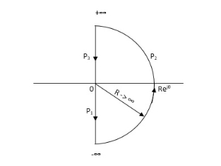
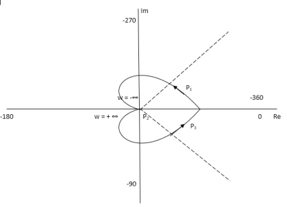
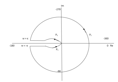
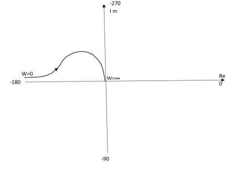
Path P1 W(0 to -∞)

M = 1/√42 + w2 √52 + w2

Φ = -tan-1(W/4) – tan-1(W/5)

W M Φ

0 1/20 00

-1 0.047 25.350

-∞ 0 +1800

Path P3 will be the mirror image across the real axis.

Path P2 :ϴ(-π/2 to 0 to +π/2)

S = Rejϴ

G(S) = 1/(Rejϴ + 4)( Rejϴ + 5)

R∞

= 1/ R2e2jϴ = 0.e-j2ϴ = 0

The plot is shown in fig 4. From plot N=0, Z=0, system stable.

Fig 4 Nyquist Plot G(S) = 1/(S + 4)(S + 5) Q3) For the given transfer function, plot the Nyquist plot and comment on stability G(S) = k/S2(S + 10)?A3) As the poles exists at origin. So, first time we do not include poles in Nyquist plot. Then check the stability for second case we include the poles at origin in Nyquist path. Then again check the stability.PART – 1: Not including poles at origin in the Nyquist Path.

Fig 5 Nyquist Path

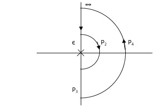
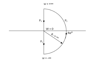
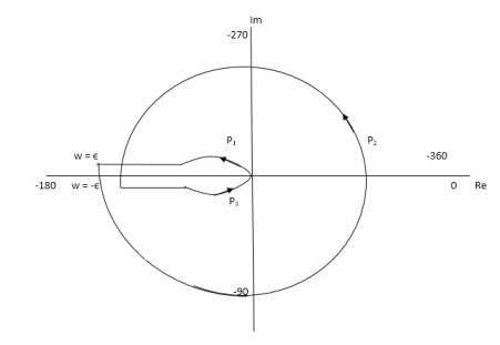
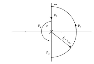
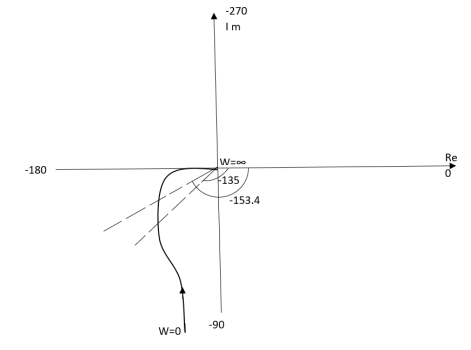
P1 W(∞ Ɛ) where Ɛ 0

P2 S = Ɛejϴ ϴ(+π/2 to 0 to -π/2)

P3 W = -Ɛ to -∞

P4 S = Rejϴ, R  ∞, ϴ = -π/2 to 0 to +π/2

For P1

M = 1/w.w√102 + w2 = 1/w2√102 + w2

Φ = -1800 – tan-1(w/10)

W M Φ

∞ 0 -3 π/2

Ɛ ∞ -1800

Path P3 will be mirror image of P1 about Real axis.

G(Ɛ ejϴ) = 1/( Ɛ ejϴ)2(Ɛ ejϴ + 10)

Ɛ 0, ϴ = π/2 to 0 to -π/2

= 1/ Ɛ2 e2jϴ(Ɛ ejϴ + 10)

= ∞. e-j2ϴ [ -2ϴ = -π to 0 to +π ]

Path P2 will be formed by rotating through -π to 0 to +π

Path P4 S = Rejϴ R  ∞ ϴ = -π/2 to 0 to +π/2

G(Rejϴ) = 1/ (Rejϴ)2(10 + Rejϴ)

= 0

N = Z – P

No poles on right half of S plane so, P = 0

N = Z – 0

Fig 6 Nyquist Plot for G(S) = k/S2(S + 10)But from plot shown in fig 6. it is clear that number of encirclements in Anticlockwise direction. So,N = 2N = Z – P2 = Z – 0Z = 2Hence, system unstable.PART 2 Including poles at origin in the Nyquist Path.

Fig 7 Nyquist PathP1 W(∞ to Ɛ) Ɛ 0P2 S = Ɛejϴ Ɛ 0 ϴ(+π/2 to +π to +3π/2)P3 W(-Ɛ to -∞) Ɛ 0P4 S = Rejϴ, R  ∞, ϴ(3π/2 to 2π to +5π/2)M = 1/W2√102 + W2 , φ = - π – tan-1(W/10)P1 W(∞ to Ɛ)W M φ∞ 0 -3 π/2Ɛ ∞ -1800P3( mirror image of P1)P2 S = ƐejϴG(Ɛejϴ) = 1/ Ɛ2e2jϴ(10 + Ɛejϴ)Ɛ 0G(Ɛejϴ) = 1/ Ɛ2e2jϴ(10)= ∞. e-j2ϴϴ(π/2 to π to 3π/2)-2ϴ = (-π to -2π to -3π)P4 = 0

Fig 8 Nyquist Plot G(S) = k/S2(S + 10)The plot is shown in fig 8. from the plot it is clear that there is no encirclement of -1 in Nyquist path. (N = 0). But the two poles at origin lies to the right half of S-plane in Nyquist path.(P = 2)[see path P2]N = Z – P0 = Z – 2Z = 2Hence, system is unstable.Path P2 will be formed by rotating through -π to -2π to -3π Q4) For the transfer function T(S) = 1/S + 1 draw polar plot?A4)(1). For polar plot substitute S=jw.

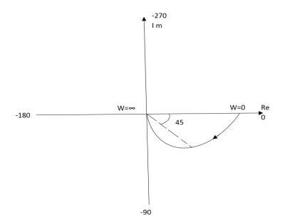
TF = 1/1 + jw

(2). Magnitude M = 1 + 0j / 1 + jw = 1/√1 + w2

(3). Phase φ = tan-1(0)/ tan-1w = - tan-1w

W M φ

0 1 00

1 0.707 -450

∞ 0 -900

The plot is shown in fig. 9(a)

Fig 9(a) Polar Plot T(S) = 1/S + 1 Q5) Plot polar plot for T(S) = 1/(S+1)(S+2)A5)

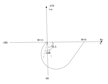
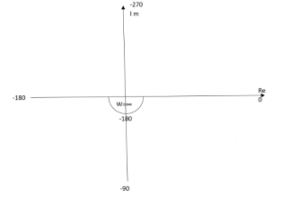
(1). S = jw

TF = 1/(1+jw)(2+jw)

(2). M = 1/(1+jw)(2+jw) = 1/-w2 + 3jw + 2

M = 1/√1 + w2√4 + w2

(3). Φ = - tan-1 w - tan-1(w/2)

W M Φ

0 0.5 00

1 0.316 -71.560

2 0.158 -108.430

∞ 0 -1800

The plot is shown in fig10(b)

Fig10(b) Polar Plot T(S) = 1/(S+1)(S+2) Intersection of polar plot with imaginary axis will be when real part of Transfer function = 0M = 1/(jw + 1)(jw + 2)= 1/-w2 + j3w + 2 Q6) Plot polar plot for T(S) = 1/SA6)(1). S = jw(2). M = 1/W(3). Φ = -tan-1(W/O) = -900W M φ0 ∞ -9001 1 -9002 0.5 -900∞ 0 -900The plot is shown in fig.11(a)

Fig 11(a) Polar Plot T(S) = 1/S Q7) Plot polar plot for T(S) = 1/S2A7)(1). S = jw(2). M = 1/w2(3). Φ = -tan-1(W/O)-tan-1(W/O) = -1800W M Φ0 ∞ -18001 1 -18002 0.25 -1800∞ 0 -1800The plot is shown in fig.12(b)

Fig 12(b) Polar Plot T(S) = 1/S2Q8) Plot polar plot for T(S) = 1/S(S+1)A8)(1). M = 1/W√1+w2(2). Φ = -900 - tan -1(W/T)W M φ0 ∞ -9001 0.707 -13502 0.45 -153.40∞ 0 -1800The plot is shown in fig.13(a)

Fig 13(a) Polar Plot T(S) = 1/S(S+1) Q9) Plot polar plot for T(s) = 1/S2(S+1)A9)(1). M = 1/w2√1+jw(2). Φ = -1800 – tan-1W/TThe plot is shown in fig.14(b)

Fig 14(b) Polar Plot T(s) = 1/S2(S+1)Q10) Explain mapping in Nyquist Plot?A10) q(S) = 1 + G(S)G(S) is always given to us, so we can relate G(S) with q(S).G(S) = q(S) – 1But q(S) can be drawn by adding 1 real part to the q(S).

Fig 15 MappingG(S) given then q(S) shift to right side.

Sign Up